Suppose the data is generated in this way: x is from random normal with mean 0, std = 10. length of x is 1000.
-
if x < -15, then y = -2 · x + 3
-
if -15 < x < 10, then y = x + 48
-
if x < 10, then y = -4 · x + 98
We can rewrite the above funcion in the following way:
\(y = \alpha + \beta_1 \times x + \beta_2 \times (x + 15) I(x > -15) + \beta_3 \times (x - 10) I(x > 10)\)
\(y = 3 - 2 \times x + 3 \times (x + 15) I(x > -15) - 5 \times (x - 10) I(x > 10)\)
python code to generate the simulation data. In different intervals of x, the relation between x and y is different.
import pandas as pd
import numpy as np
import matplotlib.pyplot as plt
import statsmodels.formula.api as smf

# plot inline rather than pop out
%matplotlib inline
# change the plot size, default is (6, 4) which is a little small
plt.rcParams['figure.figsize'] = (16, 12)

np.random.seed(9999)
x = np.random.normal(0, 1, 1000) * 10
y = np.where(x < -15, -2 * x + 3 , np.where(x < 10, x + 48, -4 * x + 98)) + np.random.normal(0, 3, 1000)
plt.scatter(x, y, s = 5, color = u'b', marker = '.', label = 'scatter plt')
plt.show()
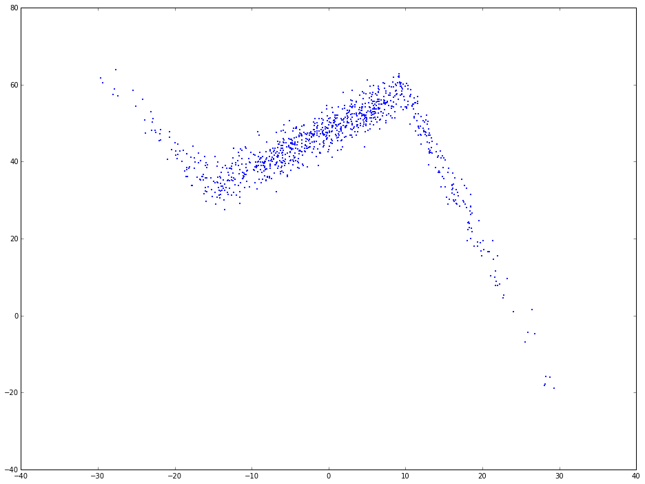
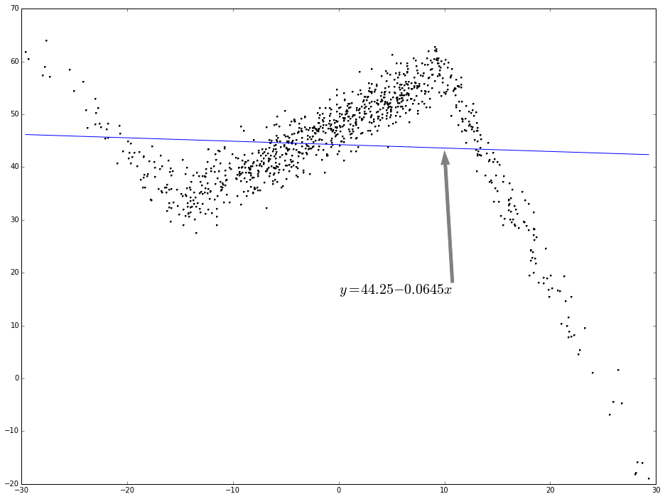
As you can see, the relation between x and y is not simplely linear. If use linear regression to fit this, the regression line will be like the following:
# linear regression
f1 = smf.ols(formula = 'y ~ x', data = dtest).fit()
dtest['f1_pred'] = f1.predict()
# print f1.summary()

fig = plt.figure()
fig.patch.set_alpha = 0.5

ax = fig.add_subplot(111)
ax.plot(x, y, linestyle = '', color = 'k', linewidth = 0.25, markeredgecolor='none', marker = '.', label = r'scatter plot')
ax.plot(dtest.x, dtest.f1_pred, color = 'blue', linestyle = '-', linewidth = 1, markeredgecolor='none', marker = '', label = r'lin-reg')
ax.annotate('$y = 44.25 - 0.0645 x$', (10, 43), xytext = (0.5, 0.4), fontsize = 20, textcoords = 'axes fraction',  arrowprops = dict(facecolor = 'grey', color = 'grey'))
plt.show()
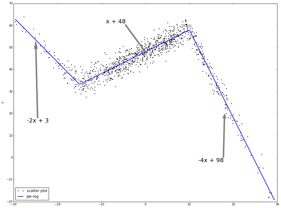
Piecewise linear regression:
-
for each interval, a linear line will be fitted.
-
the fitting function is continuous at the change points.
As is shown, the piecewise linear regression fits the data much better than linear regression directly.
# piecewise linear data prepare
x1 = np.where(x > -15, x + 15, 0)
x2 = np.where(x > 10, x - 10, 0)
dtest = pd.DataFrame([y, x, x1, x2]).T
dtest.columns = ['y', 'x', 'x1', 'x2']

# piecewise linear regression
f2 = smf.ols(formula = 'y ~ x + x1 + x2', data = dtest).fit()
dtest['f2_pred'] = f2.predict()
# print f2.summary()

dtest.sort('x', inplace = True)

fig = plt.figure(figsize = (16, 12))

ax = fig.add_subplot(111)

ax.plot(x, y, linestyle = '', color = 'k', linewidth = 0.25, markeredgecolor='none', marker = '.', label = r'scatter plot')
ax.plot(dtest.x, dtest.f2_pred, color = 'b', linestyle = '-', linewidth = 2, markeredgecolor='none', marker = '', label = r'pw-reg')
ax.set_ylabel('Y', labelpad = 6)

# pd.DataFrame([x, f2_pred]).to_excel(r'c:\test.xlsx')

ax.annotate('-2x + 3', (-25, 53), xytext = (-.95, 0.4), fontsize = 20, textcoords = 'axes fraction', arrowprops = dict(facecolor = 'grey', color = 'grey'))
ax.annotate('x + 48', (0, 48), xytext = (0.35, 0.9), fontsize = 20, textcoords = 'axes fraction', arrowprops = dict(facecolor = 'grey', color = 'grey'))
ax.annotate('-4x + 98', (18, 20), xytext = (0.7, 0.2), fontsize = 20, textcoords = 'axes fraction', arrowprops = dict(facecolor = 'grey', color = 'grey'))


plt.legend(loc = 3, ncol = 1)

plt.show()
Using np.piecewise
np.piecewise will evaluate a piecewise-defined function. After the piecewise linear function is defined, we can use optimize.curve_fit to find the optimized solution to the parameters. The benefit is you don't need to define the cutoff point. It will automatically solve the function: finding both the coefficients and the cutoff points.
from scipy import optimize

def piecewise_linear(x, x0, x1, b, k1, k2, k3):
    condlist = [x < x0, (x >= x0) & (x < x1), x >= x1]
    funclist = [lambda x: k1*x + b, lambda x: k1*x + b + k2*(x-x0), lambda x: k1*x + b + k2*(x-x0) + k3*(x - x1)]
    return np.piecewise(x, condlist, funclist)

p , e = optimize.curve_fit(piecewise_linear, x, y)

xd = np.linspace(-30, 30, 1000)
plt.plot(x, y, "o")
plt.plot(xd, piecewise_linear(xd, *p))