1 - Simple and Multiple Regression
Outline
1.0 Introduction
1.1 A First Regression Analysis
1.2 Multiple regression
1.3 Data Analysis / Examining Data
1.4 Summary
1.5 For more information / Reference
1.0 Introduction
This first Chapter will cover topics in simple and multiple regression, as well as the supporting tasks that are important in preparing to analyze your data, e.g., data checking, getting familiar with your data file, and examining the distribution of your variables. We will illustrate the basics of simple and multiple regression and demonstrate the importance of inspecting, checking and verifying your data before accepting the results of your analysis.
In this chapter, and in subsequent chapters, I will be using a data file called elemapi from the California Department of Education's API 2000 dataset. This data file contains a measure of school academic performance as well as other attributes of the elementary schools, such as, class size, enrollment, poverty, etc.
1.1 A First Regression Analysis
Let's dive right in and perform a regression analysis using the variables api00, acs_k3, meals and full. These measure the academic performance of the school (api00), the average class size in kindergarten through 3rd grade (acs_k3), the percentage of students receiving free meals (meals) - which is an indicator of poverty, and the percentage of teachers who have full teaching credentials (full). We expect that better academic performance would be associated with lower class size, fewer students receiving free meals, and a higher percentage of teachers having full teaching credentials.
First I will import some of the necessary modules in python. Typically I will use statsmodels here whose result is the same as lm in R. sklearn is very popular in data mining considering speed but its result will be different from R or SAS.
import pandas as pd
import numpy as np
import itertools
from itertools import chain, combinations
import statsmodels.formula.api as smf
import scipy.stats as scipystats
import statsmodels.api as sm
import statsmodels.stats.stattools as stools
import statsmodels.stats as stats
from statsmodels.graphics.regressionplots import *
import matplotlib.pyplot as plt
import seaborn as sns
import copy
from sklearn.cross_validation import train_test_split
import math
import time

%matplotlib inline
plt.rcParams['figure.figsize'] = (16, 12)

mypath =  r'D:\Dropbox\ipynb_download\ipynb_blog\\'

elemapi = pd.read_pickle(mypath + r'elemapi.pkl')

print elemapi[['api00', 'acs_k3', 'meals',  'full']].head()
   api00  acs_k3  meals  full
0    693    16.0   67.0  76.0
1    570    15.0   92.0  79.0
2    546    17.0   97.0  68.0
3    571    20.0   90.0  87.0
4    478    18.0   89.0  87.0
There are different way to run linear regression in statsmodels. One is using formula as R did. Another one is input the data directly. I will show them both here. And both of them will give the same result.
Personally I prefer the first way, the reasons are:
-
If we use the second way(
sm.OLS) to run the model, by default, it does not include intercept part in the model. To include intercept, we need to manually add constant to the data bysm.add_constant. -
the first way will take care of the missing data while the second will not.
'''
1. using formula as R did
'''
print '-'*40 + ' smf.ols in R formula ' + '-'*40 + '\n'
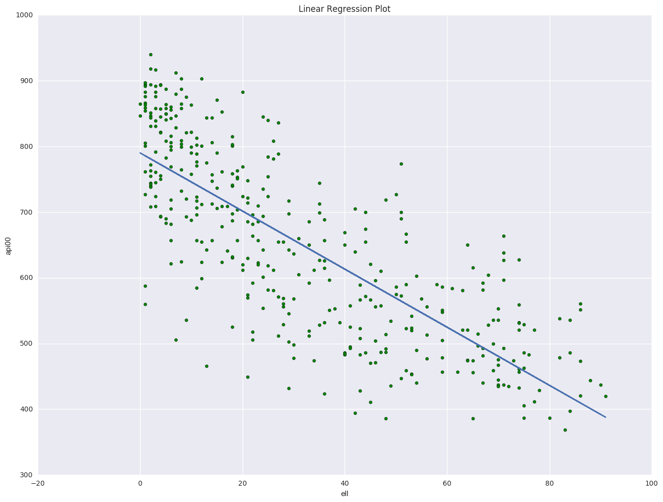
lm = smf.ols(formula = 'api00 ~ ell', data = elemapi).fit()
print lm.summary()
plt.figure()
plt.scatter(elemapi.ell, elemapi.api00, c = 'g')
plt.plot(elemapi.ell, lm.params[0] + lm.params[1] * elemapi.ell)
plt.xlabel('ell')
plt.ylabel('api00')
plt.title("Linear Regression Plot")
---------------------------------------- smf.ols in R formula ----------------------------------------

                            OLS Regression Results
==============================================================================
Dep. Variable:                  api00   R-squared:                       0.604
Model:                            OLS   Adj. R-squared:                  0.603
Method:                 Least Squares   F-statistic:                     582.3
Date:                Tue, 27 Dec 2016   Prob (F-statistic):           8.06e-79
Time:                        15:10:45   Log-Likelihood:                -2272.4
No. Observations:                 384   AIC:                             4549.
Df Residuals:                     382   BIC:                             4557.
Df Model:                           1
Covariance Type:            nonrobust
==============================================================================
                 coef    std err          t      P>|t|      [95.0% Conf. Int.]
------------------------------------------------------------------------------
Intercept    790.1777      7.428    106.375      0.000       775.572   804.783
ell           -4.4213      0.183    -24.132      0.000        -4.782    -4.061
==============================================================================
Omnibus:                        7.163   Durbin-Watson:                   1.505
Prob(Omnibus):                  0.028   Jarque-Bera (JB):                7.192
Skew:                          -0.308   Prob(JB):                       0.0274
Kurtosis:                       2.737   Cond. No.                         65.5
==============================================================================

Warnings:
[1] Standard Errors assume that the covariance matrix of the errors is correctly specified.


<matplotlib.text.Text at 0x25792668>
'''
2. using data input directly
'''
print '-'*40 + ' sm.OLS with direct input data ' + '-'*40 + '\n'
lm2 = sm.OLS(elemapi['api00'], sm.add_constant(elemapi[['ell']])).fit()
print lm2.summary()
---------------------------------------- sm.OLS with direct input data ----------------------------------------

                            OLS Regression Results
==============================================================================
Dep. Variable:                  api00   R-squared:                       0.604
Model:                            OLS   Adj. R-squared:                  0.603
Method:                 Least Squares   F-statistic:                     582.3
Date:                Tue, 20 Dec 2016   Prob (F-statistic):           8.06e-79
Time:                        21:13:43   Log-Likelihood:                -2272.4
No. Observations:                 384   AIC:                             4549.
Df Residuals:                     382   BIC:                             4557.
Df Model:                           1
Covariance Type:            nonrobust
==============================================================================
                 coef    std err          t      P>|t|      [95.0% Conf. Int.]
------------------------------------------------------------------------------
const        790.1777      7.428    106.375      0.000       775.572   804.783
ell           -4.4213      0.183    -24.132      0.000        -4.782    -4.061
==============================================================================
Omnibus:                        7.163   Durbin-Watson:                   1.505
Prob(Omnibus):                  0.028   Jarque-Bera (JB):                7.192
Skew:                          -0.308   Prob(JB):                       0.0274
Kurtosis:                       2.737   Cond. No.                         65.5
==============================================================================

Warnings:
[1] Standard Errors assume that the covariance matrix of the errors is correctly specified.
1.2 Multiple variable regression
Most of the time one variable in the model will not give us enough power to use. Usually multiple variables will be used in the model. As described about, let's try 3 variables in the model.
'''
1. using formula as R did
'''
lm = smf.ols(formula = 'api00 ~ acs_k3 + meals + full', data = elemapi).fit()
print lm.summary()
                            OLS Regression Results
==============================================================================
Dep. Variable:                  api00   R-squared:                       0.669
Model:                            OLS   Adj. R-squared:                  0.666
Method:                 Least Squares   F-statistic:                     198.7
Date:                Tue, 20 Dec 2016   Prob (F-statistic):           1.76e-70
Time:                        17:07:12   Log-Likelihood:                -1670.8
No. Observations:                 299   AIC:                             3350.
Df Residuals:                     295   BIC:                             3364.
Df Model:                           3
Covariance Type:            nonrobust
==============================================================================
                 coef    std err          t      P>|t|      [95.0% Conf. Int.]
------------------------------------------------------------------------------
Intercept    908.5016     28.887     31.451      0.000       851.652   965.351
acs_k3        -2.7820      1.420     -1.959      0.051        -5.577     0.013
meals         -3.7020      0.160    -23.090      0.000        -4.018    -3.386
full           0.1214      0.093      1.299      0.195        -0.063     0.305
==============================================================================
Omnibus:                        1.986   Durbin-Watson:                   1.463
Prob(Omnibus):                  0.370   Jarque-Bera (JB):                1.971
Skew:                           0.141   Prob(JB):                        0.373
Kurtosis:                       2.719   Cond. No.                         750.
==============================================================================

Warnings:
[1] Standard Errors assume that the covariance matrix of the errors is correctly specified.
however, if I rum sm.OLS(elemapi['api00'], sm.add_constant(elemapi[['acs_k3', 'meals', 'full']])).fit() I will get errors like "LinAlgError: SVD did not converge". The reason is there are missing data in 'acs_k3' and 'meals'. Thus results in the singular value decomposition of the hat matrix failed. To fix it, I need to drop any row with missing data first. After that, it will run successfully and the result is exactly the same as above.
'''
2. using data input directly
'''
data = elemapi[['api00', 'acs_k3', 'meals',  'full']]
data = data.dropna(axis = 0, how = 'any')

lm2 = sm.OLS(data['api00'], sm.add_constant(data[['acs_k3', 'meals',  'full']])).fit()
print lm2.summary()
                            OLS Regression Results
==============================================================================
Dep. Variable:                  api00   R-squared:                       0.669
Model:                            OLS   Adj. R-squared:                  0.666
Method:                 Least Squares   F-statistic:                     198.7
Date:                Tue, 20 Dec 2016   Prob (F-statistic):           1.76e-70
Time:                        17:10:47   Log-Likelihood:                -1670.8
No. Observations:                 299   AIC:                             3350.
Df Residuals:                     295   BIC:                             3364.
Df Model:                           3
Covariance Type:            nonrobust
==============================================================================
                 coef    std err          t      P>|t|      [95.0% Conf. Int.]
------------------------------------------------------------------------------
const        908.5016     28.887     31.451      0.000       851.652   965.351
acs_k3        -2.7820      1.420     -1.959      0.051        -5.577     0.013
meals         -3.7020      0.160    -23.090      0.000        -4.018    -3.386
full           0.1214      0.093      1.299      0.195        -0.063     0.305
==============================================================================
Omnibus:                        1.986   Durbin-Watson:                   1.463
Prob(Omnibus):                  0.370   Jarque-Bera (JB):                1.971
Skew:                           0.141   Prob(JB):                        0.373
Kurtosis:                       2.719   Cond. No.                         750.
==============================================================================

Warnings:
[1] Standard Errors assume that the covariance matrix of the errors is correctly specified.
1.3 Data Analysis
Generally, when we get the data we will do some analysis of the data.
For numeric data, we will usualy do:
- if there is any missing data
- what is the distribution of the data, and its visualization like histogram and box-plot
- what is the five numbers: min, 25 percentile, median, 75 percentile, and the max
- mean, stdev, length
- the correlation between the data
- futuremore, is there any outliers in the data?
- other plots: pairwise scatter plot, kernal density plot
For categorical data, we will usually do:
- is there any missing data?
- how many unique values of the data? what is their frequency?
Next we will answer these questions.
we will pick 4 variables from the elemapi data as an example.
1.3.1. The df.describe() will gives the summary information like how many non-missing values there, mean, stdev, and the five number summary.
As we can see, api00 and full does not have missing values and their length is 384. acs_k3 has 382 non-missing values, so it has two missing data. meals has 301 non-missing values so it has 83 missings.
sample_data = elemapi[['api00', 'acs_k3', 'meals',  'full']]
print sample_data.describe()
            api00      acs_k3       meals        full
count  384.000000  382.000000  301.000000  384.000000
mean   649.421875   18.534031   71.890365   65.124271
std    143.020564    5.104436   24.367696   40.823987
min    369.000000  -21.000000    6.000000    0.420000
25%    525.000000         NaN         NaN    0.927500
50%    646.500000         NaN         NaN   87.000000
75%    763.500000         NaN         NaN   97.000000
max    940.000000   25.000000  100.000000  100.000000
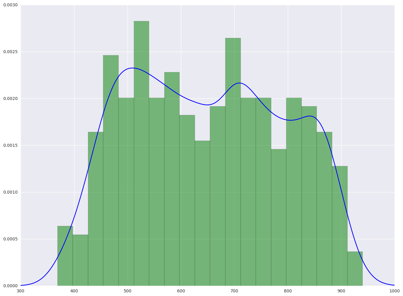
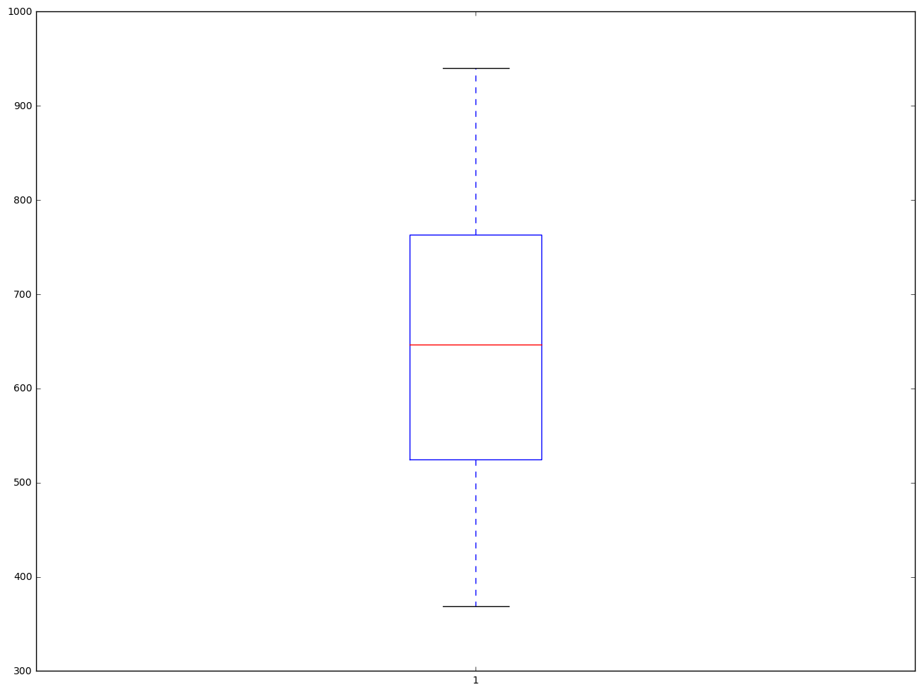
1.3.2. plot the histogram and the density plot
From the hist plot, the data api00 is pretty even. There is no special concentration.
From the box plot below, we did not see there is any outliers.
from scipy.stats import gaussian_kde

plt.hist(elemapi.api00, 20, normed = 1, facecolor = 'g', alpha = 0.5)

# add density plot
density = gaussian_kde(elemapi.api00)
xs = np.linspace(300, 1000, 500)
density.covariance_factor = lambda : .2
density._compute_covariance()
plt.plot(xs, density(xs), color = "b")
plt.show()
plt.boxplot(elemapi.api00, 0, 'gD')
{'boxes': [<matplotlib.lines.Line2D at 0x18adfb00>],
 'caps': [<matplotlib.lines.Line2D at 0x18af37b8>,
  <matplotlib.lines.Line2D at 0x18af3d30>],
 'fliers': [<matplotlib.lines.Line2D at 0x18aff860>],
 'means': [],
 'medians': [<matplotlib.lines.Line2D at 0x18aff2e8>],
 'whiskers': [<matplotlib.lines.Line2D at 0x18adfc18>,
  <matplotlib.lines.Line2D at 0x18af3240>]}
1.3.3. The correlation of the data
df.corr() will give the correlation matrix of all the variables. Pick the corresponding row or column will give us the correlation between that variables with all the other variables.
# check correlation between each variable and api00
print elemapi.corr().ix['api00', :].sort_values()
mealcat    -0.865752
meals      -0.815576
ell        -0.777091
not_hsg    -0.681712
emer       -0.596273
yr_rnd     -0.487599
hsg        -0.361842
enroll     -0.329078
mobility   -0.191732
growth     -0.102593
acs_k3     -0.095982
dnum        0.007991
acs_46      0.223256
some_col    0.258125
snum        0.259491
full        0.424186
col_grad    0.529277
grad_sch    0.632367
avg_ed      0.793012
api99       0.985950
api00       1.000000
Name: api00, dtype: float64
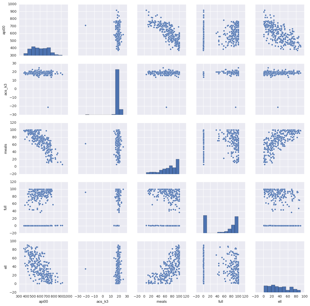
1.3.4. scatter plot of all the variables in the data
This will scatter plot all the pairs of the data so that we can easily find their relations. If there is too many variables, this is not a good way because there are too many graphs to display. In that case, the correlation will be easier to check.
sns.pairplot(elemapi[['api00', 'acs_k3', 'meals', 'full', 'ell']].dropna(how = 'any', axis = 0))
<seaborn.axisgrid.PairGrid at 0x1d83e6d8>
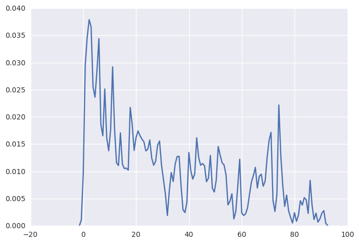
1.3.5. keneral density plot
R has a very friendly function plot(density(data, bw=0.5)) to let us plot the kernal density function. Here is try to mimic that in python. From the plot we can observe that the ell variable skewed to the right.
sns.kdeplot(np.array(elemapi.ell), bw=0.5)
<matplotlib.axes._subplots.AxesSubplot at 0x25336f98>
1.3.6. categorical variable frequency
For categorical variable, most of the time we care about if there is any missing data, and what is the frequency of the values. We can see for acs_k3, there are about 137 data points equal to 19.
elemapi.acs_k3.value_counts(dropna = False).sort_index()
-21.0      3
-20.0      2
-19.0      1
 14.0      2
 15.0      1
 16.0     14
 17.0     19
 18.0     59
 19.0    137
 20.0     94
 21.0     39
 22.0      7
 23.0      3
 25.0      1
NaN        2
Name: acs_k3, dtype: int64
1.4 Summary
Most of the time, when I get the data, I will do single variable analysis to check the distribution of my data and missing information. If data is not big, I will check the pairwise relations by pairwise scatter plot or the correlations.
If there is missing, how to do? Drop the data or consider of any way to impute the missingt data?
If the relation is not linear, what shall we do?
1.5 For more information
If you have any suggestions, please contact me.
Some references that I think may help:
-
Applied Linear Statistical Models. I have a hard copy of this book which I bought in XJTU library. It only costs about two US Dollars
-
UCLA ATS: regression with SAS. Although it uses SAS, it gives very detailed introduction about linear models. I will follow the structure of this web book.
-
statsmodels A python package to run statistical models and tests.