2 - Regression Diagnostics
Outline
2.0 Regression Diagnostics
2.1 Unusual and Influential data
2.2 Tests on Normality of Residuals
2.3 Tests on Nonconstant Error of Variance
2.4 Tests on Multicollinearity
2.5 Tests on Nonlinearity
2.6 Model Specification
2.7 Issues of Independence
2.8 Summary
2.9 For more information
2.0 Regression Diagnostics
When run regression models, you need to do regression disgnostics. Without verifying that your data have met the regression assumptions, your results may be misleading. This section will explore how to do regression diagnostics.
- Linearity - the relationships between the predictors and the outcome variable should be linear
- Normality - the errors should be normally distributed - technically normality is necessary only for the t-tests to be valid, estimation of the coefficients only requires that the errors be identically and independently distributed
- Homogeneity of variance (homoscedasticity) - the error variance should be constant
- Independence - the errors associated with one observation are not correlated with the errors of any other observation
- Errors in variables - predictor variables are measured without error (we will cover this in Chapter 4)
- Model specification - the model should be properly specified (including all relevant variables, and excluding irrelevant variables)
Additionally, there are issues that can arise during the analysis that, while strictly speaking, are not assumptions of regression, are none the less, of great concern to regression analysts.
- Influence - individual observations that exert undue influence on the coefficients
- Collinearity - predictors that are highly collinear, i.e. linearly related, can cause problems in estimating the regression coefficients.
2.1 Unusual and influential data
A single observation that is substantially different from all other observations can make a large difference in the results of your regression analysis. If a single observation (or small group of observations) substantially changes your results, you would want to know about this and investigate further. There are three ways that an observation can be unusual.
Outliers: In linear regression, an outlier is an observation with large residual. In other words, it is an observation whose dependent-variable value is unusual given its values on the predictor variables. An outlier may indicate a sample peculiarity or may indicate a data entry error or other problem.
Leverage: An observation with an extreme value on a predictor variable is called a point with high leverage. Leverage is a measure of how far an observation deviates from the mean of that variable. These leverage points can have an effect on the estimate of regression coefficients.
Influence: An observation is said to be influential if removing the observation substantially changes the estimate of coefficients. Influence can be thought of as the product of leverage and outlierness.
How can we identify these three types of observations? Let's look at an example dataset called crime. This dataset appears in Statistical Methods for Social Sciences, Third Edition by Alan Agresti and Barbara Finlay (Prentice Hall, 1997). The variables are state id (sid), state name (state), violent crimes per 100,000 people (crime), murders per 1,000,000 (murder), the percent of the population living in metropolitan areas (pctmetro), the percent of the population that is white (pctwhite), percent of population with a high school education or above (pcths), percent of population living under poverty line (poverty), and percent of population that are single parents (single).
import pandas as pd
import numpy as np
import itertools
from itertools import chain, combinations
import statsmodels.formula.api as smf
import scipy.stats as scipystats
import statsmodels.api as sm
import statsmodels.stats.stattools as stools
import statsmodels.stats as stats
from statsmodels.graphics.regressionplots import *
import matplotlib.pyplot as plt
import seaborn as sns
import copy
from sklearn.cross_validation import train_test_split
import math
import time

%matplotlib inline
plt.rcParams['figure.figsize'] = (16, 12)

mypath =  r'D:\Dropbox\ipynb_download\ipynb_blog\\'

crime = pd.read_csv(mypath + r'crime.csv')
crime.describe()
| sid | crime | murder | pctmetro | pctwhite | pcths | poverty | single | |
|---|---|---|---|---|---|---|---|---|
| count | 51.000000 | 51.000000 | 51.000000 | 51.000000 | 51.000000 | 51.000000 | 51.000000 | 51.000000 |
| mean | 26.000000 | 612.843137 | 8.727451 | 67.390196 | 84.115686 | 76.223529 | 14.258824 | 11.325490 |
| std | 14.866069 | 441.100323 | 10.717576 | 21.957133 | 13.258392 | 5.592087 | 4.584242 | 2.121494 |
| min | 1.000000 | 82.000000 | 1.600000 | 24.000000 | 31.800000 | 64.300000 | 8.000000 | 8.400000 |
| 25% | 13.500000 | 326.500000 | 3.900000 | 49.550000 | 79.350000 | 73.500000 | 10.700000 | 10.050000 |
| 50% | 26.000000 | 515.000000 | 6.800000 | 69.800000 | 87.600000 | 76.700000 | 13.100000 | 10.900000 |
| 75% | 38.500000 | 773.000000 | 10.350000 | 83.950000 | 92.600000 | 80.100000 | 17.400000 | 12.050000 |
| max | 51.000000 | 2922.000000 | 78.500000 | 100.000000 | 98.500000 | 86.600000 | 26.400000 | 22.100000 |
sns.pairplot(crime[['crime', 'pctmetro', 'poverty', 'single']].dropna(how = 'any', axis = 0))
<seaborn.axisgrid.PairGrid at 0x176314a8>
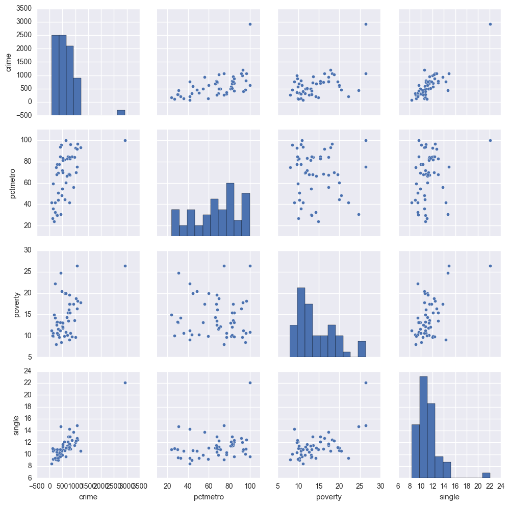
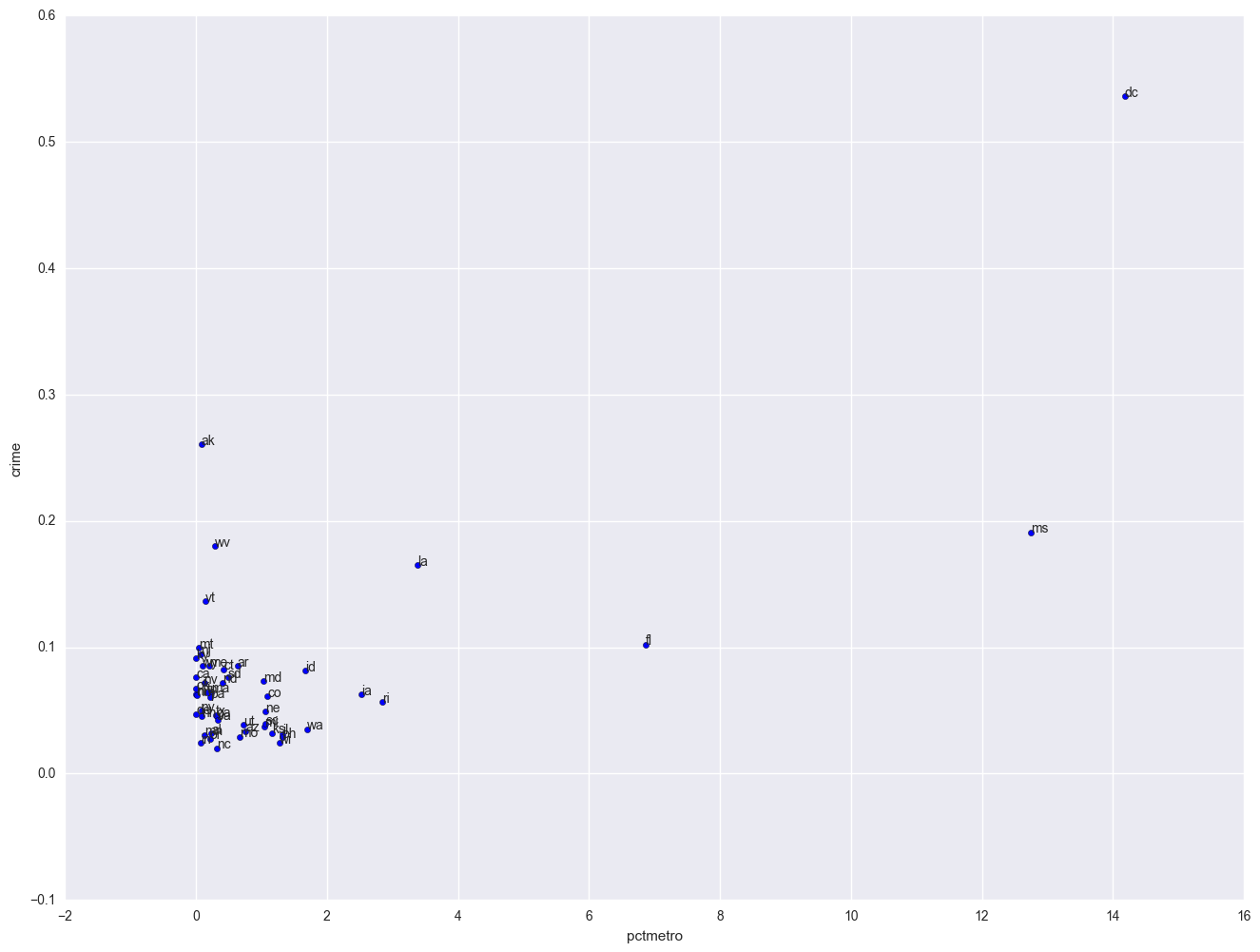
The graphs of crime with other variables show some potential problems. In every plot, we see a data point that is far away from the rest of the data points. Let's make individual graphs of crime with pctmetro and poverty and single so we can get a better view of these scatterplots. We will add the label plot of the state name instead of a point.
plt.scatter(crime.pctmetro, crime.crime)

for i, state in enumerate(crime.state):
    plt.annotate(state, [crime.pctmetro[i], crime.crime[i]])

plt.xlabel("pctmetro")
plt.ylabel("crime")
<matplotlib.text.Text at 0x130b47f0>
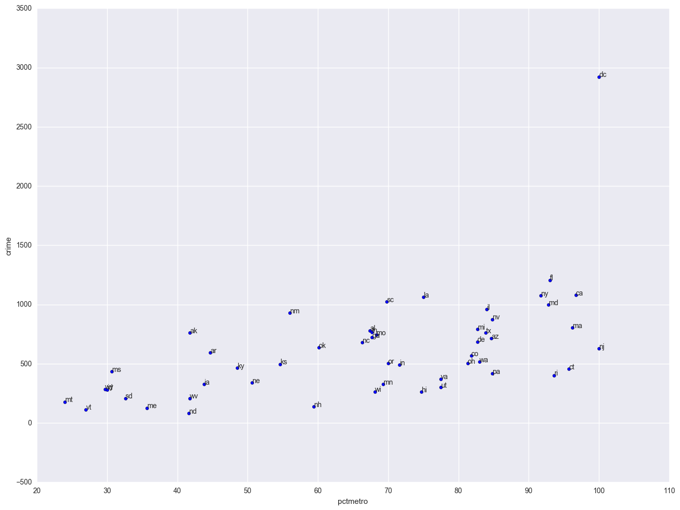
All the scatter plots suggest that the observation for state = dc is a point that requires extra attention since it stands out away from all of the other points. We will keep it in mind when we do our regression analysis.
Now let's try the regression predicting crime from pctmetro, poverty and single. We will go step-by-step to identify all the potentially unusual or influential points afterwards. We will output several statistics that we will need for the next few analyses to a dataset called crime1res, and we will explain each statistic in turn. These statistics include the studentized residual (called resid_student), leverage (called leverage), Cook's D (called cooks) and DFFITS (called dffits). We are requesting all of these statistics now so that they can be placed in a single dataset that we will use for the next several examples.
pd.Series(influence.hat_matrix_diag).describe()
count    51.000000
mean      0.078431
std       0.080285
min       0.020061
25%       0.037944
50%       0.061847
75%       0.083896
max       0.536383
dtype: float64
lm = smf.ols(formula = "crime ~ pctmetro + poverty + single", data = crime).fit()
print lm.summary()
influence = lm.get_influence()
resid_student = influence.resid_studentized_external
(cooks, p) = influence.cooks_distance
(dffits, p) = influence.dffits
leverage = influence.hat_matrix_diag
print '\n'
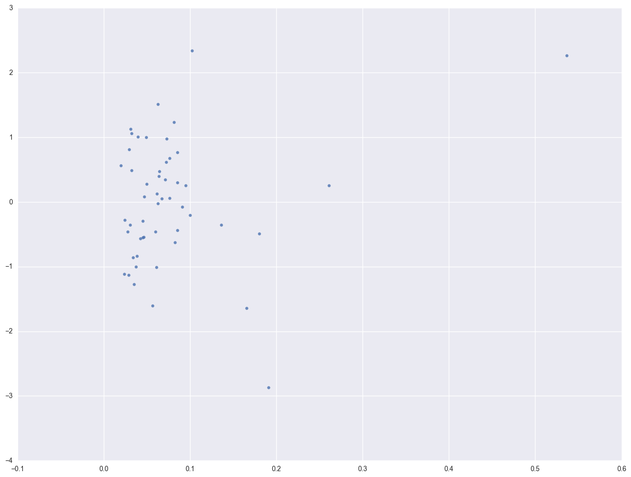
print 'Leverage v.s. Studentized Residuals'
sns.regplot(leverage, lm.resid_pearson, fit_reg=False)
                            OLS Regression Results
==============================================================================
Dep. Variable:                  crime   R-squared:                       0.840
Model:                            OLS   Adj. R-squared:                  0.830
Method:                 Least Squares   F-statistic:                     82.16
Date:                Mon, 26 Dec 2016   Prob (F-statistic):           1.03e-18
Time:                        07:12:55   Log-Likelihood:                -335.71
No. Observations:                  51   AIC:                             679.4
Df Residuals:                      47   BIC:                             687.1
Df Model:                           3
Covariance Type:            nonrobust
==============================================================================
                 coef    std err          t      P>|t|      [95.0% Conf. Int.]
------------------------------------------------------------------------------
Intercept  -1666.4359    147.852    -11.271      0.000     -1963.876 -1368.996
pctmetro       7.8289      1.255      6.240      0.000         5.305    10.353
poverty       17.6802      6.941      2.547      0.014         3.717    31.644
single       132.4081     15.503      8.541      0.000       101.220   163.597
==============================================================================
Omnibus:                        2.081   Durbin-Watson:                   1.706
Prob(Omnibus):                  0.353   Jarque-Bera (JB):                1.284
Skew:                          -0.093   Prob(JB):                        0.526
Kurtosis:                       3.755   Cond. No.                         424.
==============================================================================

Warnings:
[1] Standard Errors assume that the covariance matrix of the errors is correctly specified.


Leverage v.s. Studentized Residuals


<matplotlib.axes._subplots.AxesSubplot at 0x1baf2f28>
crime1res = pd.concat([pd.Series(cooks, name = "cooks"), pd.Series(dffits, name = "dffits"), pd.Series(leverage, name = "leverage"), pd.Series(resid_student, name = "resid_student")], axis = 1)
crime1res = pd.concat([crime, crime1res], axis = 1)
crime1res.head()
| sid | state | crime | murder | pctmetro | pctwhite | pcths | poverty | single | cooks | dffits | leverage | resid_student | |
|---|---|---|---|---|---|---|---|---|---|---|---|---|---|
| 0 | 1 | ak | 761 | 9.0 | 41.8 | 75.2 | 86.6 | 9.1 | 14.3 | 0.007565 | 0.172247 | 0.260676 | 0.290081 |
| 1 | 2 | al | 780 | 11.6 | 67.4 | 73.5 | 66.9 | 17.4 | 11.5 | 0.002020 | 0.089166 | 0.032089 | 0.489712 |
| 2 | 3 | ar | 593 | 10.2 | 44.7 | 82.9 | 66.3 | 20.0 | 10.7 | 0.014897 | 0.243153 | 0.085385 | 0.795809 |
| 3 | 4 | az | 715 | 8.6 | 84.7 | 88.6 | 78.7 | 15.4 | 12.1 | 0.006654 | -0.162721 | 0.033806 | -0.869915 |
| 4 | 5 | ca | 1078 | 13.1 | 96.7 | 79.3 | 76.2 | 18.2 | 12.5 | 0.000075 | 0.017079 | 0.076468 | 0.059353 |
Let's examine the studentized residuals as a first means for identifying outliers. We requested the studentized residuals in the above regression in the output statement and named them r. Studentized residuals are a type of standardized residual that can be used to identify outliers. We see three residuals that stick out, -3.57, 2.62 and 3.77.
r = crime1res.resid_student
print '-'*30 + ' studentized residual ' + '-'*30
print r.describe()
print '\n'

r_sort = crime1res.sort_values(by = 'resid_student')
print '-'*30 + ' top 5 most negative residuals ' + '-'*30
print r_sort.head()
print '\n'

print '-'*30 + ' top 5 most positive residuals ' + '-'*30
print r_sort.tail()
------------------------------ studentized residual ------------------------------
count    51.000000
mean      0.018402
std       1.133126
min      -3.570789
25%      -0.555460
50%       0.052616
75%       0.599771
max       3.765847
Name: resid_student, dtype: float64


------------------------------ top 5 most negative residuals ------------------------------
    sid state  crime  murder  pctmetro  pctwhite  pcths  poverty  single  \
24   25    ms    434    13.5      30.7      63.3   64.3     24.7    14.7
17   18    la   1062    20.3      75.0      66.7   68.3     26.4    14.9
38   39    ri    402     3.9      93.6      92.6   72.0     11.2    10.8
46   47    wa    515     5.2      83.0      89.4   83.8     12.1    11.7
34   35    oh    504     6.0      81.3      87.5   75.7     13.0    11.4

       cooks    dffits  leverage  resid_student
24  0.602106 -1.735096  0.191012      -3.570789
17  0.159264 -0.818120  0.165277      -1.838578
38  0.041165 -0.413655  0.056803      -1.685598
46  0.015271 -0.248989  0.035181      -1.303919
34  0.009695 -0.197588  0.028755      -1.148330


------------------------------ top 5 most positive residuals ------------------------------
    sid state  crime  murder  pctmetro  pctwhite  pcths  poverty  single  \
13   14    il    960    11.4      84.0      81.0   76.2     13.6    11.5
12   13    id    282     2.9      30.0      96.7   79.7     13.1     9.5
11   12    ia    326     2.3      43.8      96.6   80.1     10.3     9.0
8     9    fl   1206     8.9      93.0      83.5   74.4     17.8    10.6
50   51    dc   2922    78.5     100.0      31.8   73.1     26.4    22.1

       cooks    dffits  leverage  resid_student
13  0.010661  0.207220  0.031358       1.151702
12  0.036675  0.385749  0.081675       1.293477
11  0.040978  0.411382  0.062768       1.589644
8   0.173629  0.883820  0.102202       2.619523
50  3.203429  4.050610  0.536383       3.765847
We should pay attention to studentized residuals that exceed +2 or -2, and get even more concerned about residuals that exceed +2.5 or -2.5 and even yet more concerned about residuals that exceed +3 or -3. These results show that DC and MS are the most worrisome observations, followed by FL.
Let's show all of the variables in our regression where the studentized residual exceeds +2 or -2, i.e., where the absolute value of the residual exceeds 2. We see the data for the three potential outliers we identified, namely Florida, Mississippi and Washington D.C. Looking carefully at these three observations, we couldn't find any data entry errors, though we may want to do another regression analysis with the extreme point such as DC deleted. We will return to this issue later.
print crime[abs(r) > 2]
    sid state  crime  murder  pctmetro  pctwhite  pcths  poverty  single
8     9    fl   1206     8.9      93.0      83.5   74.4     17.8    10.6
24   25    ms    434    13.5      30.7      63.3   64.3     24.7    14.7
50   51    dc   2922    78.5     100.0      31.8   73.1     26.4    22.1
Now let's look at the leverage's to identify observations that will have potential great influence on regression coefficient estimates.
Generally, a point with leverage greater than (2k+2)/n should be carefully examined, where k is the number of predictors and n is the number of observations. In our example this works out to (2*3+2)/51 = .15686275, so we can do the following.
leverage = crime1res.leverage
print '-'*30 + ' Leverage ' + '-'*30
print leverage.describe()
print '\n'

leverage_sort = crime1res.sort_values(by = 'leverage', ascending = False)

print '-'*30 + ' top 5 highest leverage data points ' + '-'*30
print leverage_sort.head()
------------------------------ Leverage ------------------------------
count    51.000000
mean      0.078431
std       0.080285
min       0.020061
25%       0.037944
50%       0.061847
75%       0.083896
max       0.536383
Name: leverage, dtype: float64


------------------------------ top 5 highest leverage data points ------------------------------
    sid state  crime  murder  pctmetro  pctwhite  pcths  poverty  single  \
50   51    dc   2922    78.5     100.0      31.8   73.1     26.4    22.1
0     1    ak    761     9.0      41.8      75.2   86.6      9.1    14.3
24   25    ms    434    13.5      30.7      63.3   64.3     24.7    14.7
48   49    wv    208     6.9      41.8      96.3   66.0     22.2     9.4
17   18    la   1062    20.3      75.0      66.7   68.3     26.4    14.9

       cooks    dffits  leverage  resid_student
50  3.203429  4.050610  0.536383       3.765847
0   0.007565  0.172247  0.260676       0.290081
24  0.602106 -1.735096  0.191012      -3.570789
48  0.016361 -0.253893  0.180200      -0.541535
17  0.159264 -0.818120  0.165277      -1.838578
As we have seen, DC is an observation that both has a large residual and large leverage. Such points are potentially the most influential. We can make a plot that shows the leverage by the residual squared and look for observations that are jointly high on both of these measures. We can do this using a leverage versus residual-squared plot. Using residual squared instead of residual itself, the graph is restricted to the first quadrant and the relative positions of data points are preserved. This is a quick way of checking potential influential observations and outliers at the same time. Both types of points are of great concern for us.
from statsmodels.graphics.regressionplots import *
plot_leverage_resid2(lm)
plt.show()

plt.scatter(crime1res.resid_student ** 2, crime1res.leverage)
for i, state in enumerate(crime.state):
    plt.annotate(state, [(crime1res.resid_student ** 2)[i],  crime1res.leverage[i]])
plt.xlabel("pctmetro")
plt.ylabel("crime")
plt.show()

influence_plot(lm)
plt.show()
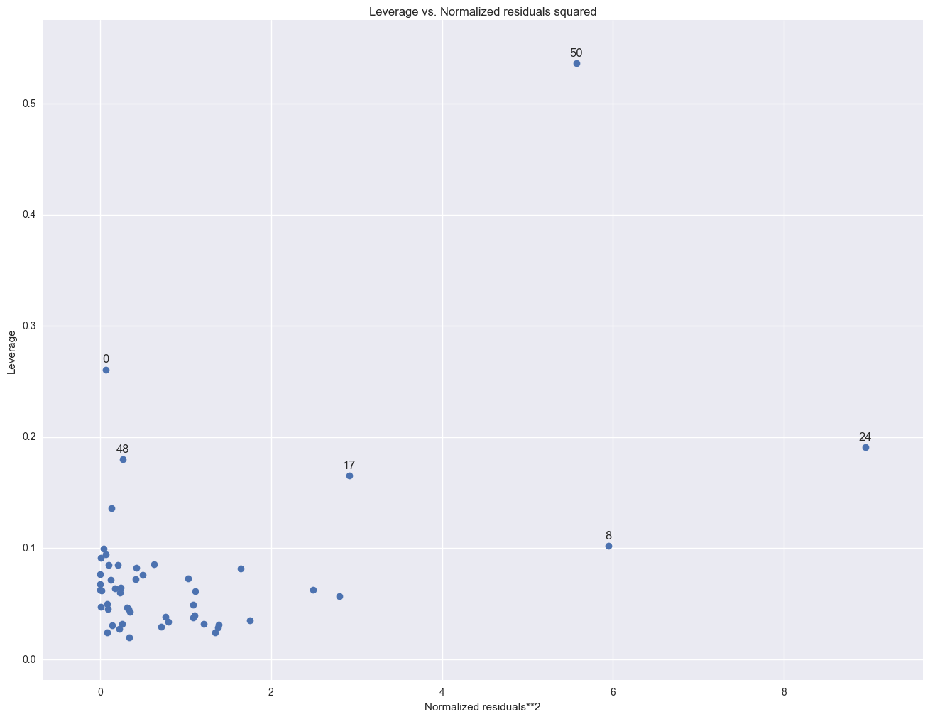
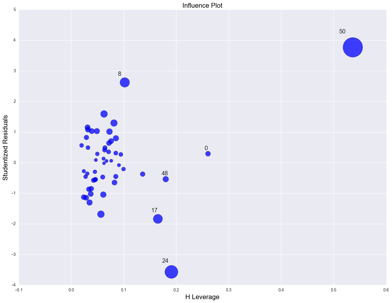
The point for DC catches our attention having both the highest residual squared and highest leverage, suggesting it could be very influential. The point for MS has almost as large a residual squared, but does not have the same leverage. We'll look at those observations more carefully by listing them below.
Now let's move on to overall measures of influence. Specifically, let's look at Cook's D and DFITS. These measures both combine information on the residual and leverage. Cook's D and DFITS are very similar except that they scale differently, but they give us similar answers.
The lowest value that Cook's D can assume is zero, and the higher the Cook's D is, the more influential the point is. The conventional cut-off point is 4/n. We can list any observation above the cut-off point by doing the following. We do see that the Cook's D for DC is by far the largest.
Now let's take a look at DFITS. The conventional cut-off point for DFITS is 2*sqrt(k/n). DFITS can be either positive or negative, with numbers close to zero corresponding to the points with small or zero influence. As we see, DFITS also indicates that DC is, by far, the most influential observation.
crime1res[abs(crime1res.dffits) > 2 * math.sqrt(3.0 / 51)]
| sid | state | crime | murder | pctmetro | pctwhite | pcths | poverty | single | cooks | dffits | leverage | resid_student | |
|---|---|---|---|---|---|---|---|---|---|---|---|---|---|
| 8 | 9 | fl | 1206 | 8.9 | 93.0 | 83.5 | 74.4 | 17.8 | 10.6 | 0.173629 | 0.883820 | 0.102202 | 2.619523 |
| 17 | 18 | la | 1062 | 20.3 | 75.0 | 66.7 | 68.3 | 26.4 | 14.9 | 0.159264 | -0.818120 | 0.165277 | -1.838578 |
| 24 | 25 | ms | 434 | 13.5 | 30.7 | 63.3 | 64.3 | 24.7 | 14.7 | 0.602106 | -1.735096 | 0.191012 | -3.570789 |
| 50 | 51 | dc | 2922 | 78.5 | 100.0 | 31.8 | 73.1 | 26.4 | 22.1 | 3.203429 | 4.050610 | 0.536383 | 3.765847 |
The above measures are general measures of influence. You can also consider more specific measures of influence that assess how each coefficient is changed by deleting the observation. This measure is called DFBETA and is created for each of the predictors. Apparently this is more computationally intensive than summary statistics such as Cook's D because the more predictors a model has, the more computation it may involve. We can restrict our attention to only those predictors that we are most concerned with and to see how well behaved those predictors are.
crimedfbeta = pd.concat([crime1res, pd.DataFrame(influence.dfbetas, columns = ['dfb_intercept', 'dfb_pctmetro', 'dfb_poverty', 'dfb_single'])], axis = 1)
print crimedfbeta.head()

# print pd.DataFrame(OLSInfluence(lm).dfbetas).head()
   sid state  crime  murder  pctmetro  pctwhite  pcths  poverty  single  \
0    1    ak    761     9.0      41.8      75.2   86.6      9.1    14.3
1    2    al    780    11.6      67.4      73.5   66.9     17.4    11.5
2    3    ar    593    10.2      44.7      82.9   66.3     20.0    10.7
3    4    az    715     8.6      84.7      88.6   78.7     15.4    12.1
4    5    ca   1078    13.1      96.7      79.3   76.2     18.2    12.5

      cooks    dffits  leverage  resid_student  dfb_intercept  dfb_pctmetro  \
0  0.007565  0.172247  0.260676       0.290081      -0.015624     -0.106185
1  0.002020  0.089166  0.032089       0.489712       0.000577      0.012429
2  0.014897  0.243153  0.085385       0.795809       0.067038     -0.068748
3  0.006654 -0.162721  0.033806      -0.869915       0.052022     -0.094761
4  0.000075  0.017079  0.076468       0.059353      -0.007311      0.012640

   dfb_poverty  dfb_single
0    -0.131340    0.145183
1     0.055285   -0.027513
2     0.175348   -0.105263
3    -0.030883    0.001242
4     0.008801   -0.003636
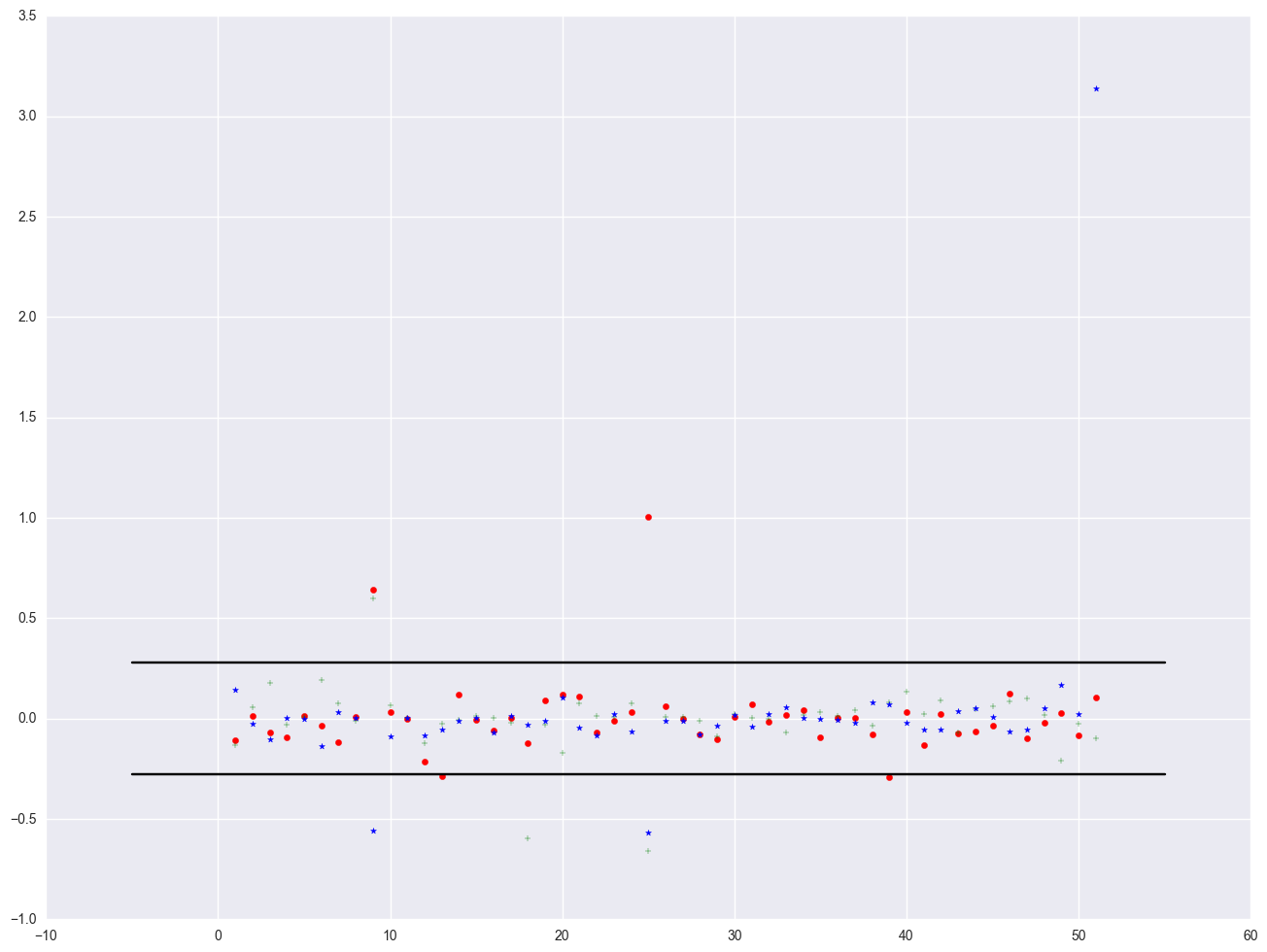
The value for DFB_single for Alaska is 0.14, which means that by being included in the analysis (as compared to being excluded), Alaska increases the coefficient for single by 0.14 standard errors, i.e., 0.14 times the standard error for BSingle or by (0.14 * 15.5). Because the inclusion of an observation could either contribute to an increase or decrease in a regression coefficient, DFBETAs can be either positive or negative. A DFBETA value in excess of 2/sqrt(n) merits further investigation. In this example, we would be concerned about absolute values in excess of 2/sqrt(51) or 0.28.
We can plot all three DFBETA values against the state id in one graph shown below. We add a line at 0.28 and -0.28 to help us see potentially troublesome observations. We see the largest value is about 3.0 for DFsingle.
plt.scatter(crimedfbeta.sid, crimedfbeta.dfb_pctmetro, color = "red", marker = "o")
plt.scatter(crimedfbeta.sid, crimedfbeta.dfb_poverty, color = "green", marker = "+")
plt.scatter(crimedfbeta.sid, crimedfbeta.dfb_single, color = "blue", marker = "*")

# add a horizontial line in pyplot, using plt.plot((x1, x2), (y1, y2), 'c-')
plt.plot((-5, 55), (0.28, 0.28), 'k-')
plt.plot((-5, 55), (-0.28, -0.28), 'k-')
[<matplotlib.lines.Line2D at 0x23161ac8>]
Finally, all the analysis showing data point with 'dc' is the most problematic observation. Let's run the regression without the 'dc' point.
lm_1 = smf.ols(formula = "crime ~ pctmetro + poverty + single", data = crime[crime.state != "dc"]).fit()
print lm_1.summary()
                            OLS Regression Results
==============================================================================
Dep. Variable:                  crime   R-squared:                       0.722
Model:                            OLS   Adj. R-squared:                  0.704
Method:                 Least Squares   F-statistic:                     39.90
Date:                Mon, 26 Dec 2016   Prob (F-statistic):           7.45e-13
Time:                        07:48:06   Log-Likelihood:                -322.90
No. Observations:                  50   AIC:                             653.8
Df Residuals:                      46   BIC:                             661.5
Df Model:                           3
Covariance Type:            nonrobust
==============================================================================
                 coef    std err          t      P>|t|      [95.0% Conf. Int.]
------------------------------------------------------------------------------
Intercept  -1197.5381    180.487     -6.635      0.000     -1560.840  -834.236
pctmetro       7.7123      1.109      6.953      0.000         5.480     9.945
poverty       18.2827      6.136      2.980      0.005         5.932    30.634
single        89.4008     17.836      5.012      0.000        53.498   125.303
==============================================================================
Omnibus:                        0.112   Durbin-Watson:                   1.760
Prob(Omnibus):                  0.945   Jarque-Bera (JB):                0.144
Skew:                           0.098   Prob(JB):                        0.930
Kurtosis:                       2.825   Cond. No.                         574.
==============================================================================

Warnings:
[1] Standard Errors assume that the covariance matrix of the errors is correctly specified.
Summary
In this section, we explored a number of methods of identifying outliers and influential points. In a typical analysis, you would probably use only some of these methods. Generally speaking, there are two types of methods for assessing outliers: statistics such as residuals, leverage, Cook's D and DFITS, that assess the overall impact of an observation on the regression results, and statistics such as DFBETA that assess the specific impact of an observation on the regression coefficients.
In our example, we found that DC was a point of major concern. We performed a regression with it and without it and the regression equations were very different. We can justify removing it from our analysis by reasoning that our model is to predict crime rate for states, not for metropolitan areas.
2.2 Tests for Normality of Residuals
One of the assumptions of linear regression analysis is that the residuals are normally distributed. This assumption assures that the p-values for the t-tests will be valid. As before, we will generate the residuals (called r) and predicted values (called fv) and put them in a dataset (called elem1res). We will also keep the variables api00, meals, ell and emer in that dataset.
Let's use the elemapi2 data file we saw in Chapter 1 for these analyses. Let's predict academic performance (api00) from percent receiving free meals (meals), percent of English language learners (ell), and percent of teachers with emergency credentials (emer).
elemapi2 = pd.read_csv(mypath + 'elemapi2.csv')
lm = smf.ols(formula = "api00 ~ meals + ell + emer", data = elemapi2).fit()
print lm.summary()

elem1res = pd.concat([elemapi2, pd.Series(lm.resid, name = 'resid'), pd.Series(lm.predict(), name = "predict")], axis = 1)
                            OLS Regression Results
==============================================================================
Dep. Variable:                  api00   R-squared:                       0.836
Model:                            OLS   Adj. R-squared:                  0.835
Method:                 Least Squares   F-statistic:                     673.0
Date:                Mon, 26 Dec 2016   Prob (F-statistic):          4.89e-155
Time:                        09:42:41   Log-Likelihood:                -2188.5
No. Observations:                 400   AIC:                             4385.
Df Residuals:                     396   BIC:                             4401.
Df Model:                           3
Covariance Type:            nonrobust
==============================================================================
                 coef    std err          t      P>|t|      [95.0% Conf. Int.]
------------------------------------------------------------------------------
Intercept    886.7033      6.260    141.651      0.000       874.397   899.010
meals         -3.1592      0.150    -21.098      0.000        -3.454    -2.865
ell           -0.9099      0.185     -4.928      0.000        -1.273    -0.547
emer          -1.5735      0.293     -5.368      0.000        -2.150    -0.997
==============================================================================
Omnibus:                        2.394   Durbin-Watson:                   1.437
Prob(Omnibus):                  0.302   Jarque-Bera (JB):                2.168
Skew:                           0.170   Prob(JB):                        0.338
Kurtosis:                       3.119   Cond. No.                         171.
==============================================================================

Warnings:
[1] Standard Errors assume that the covariance matrix of the errors is correctly specified.
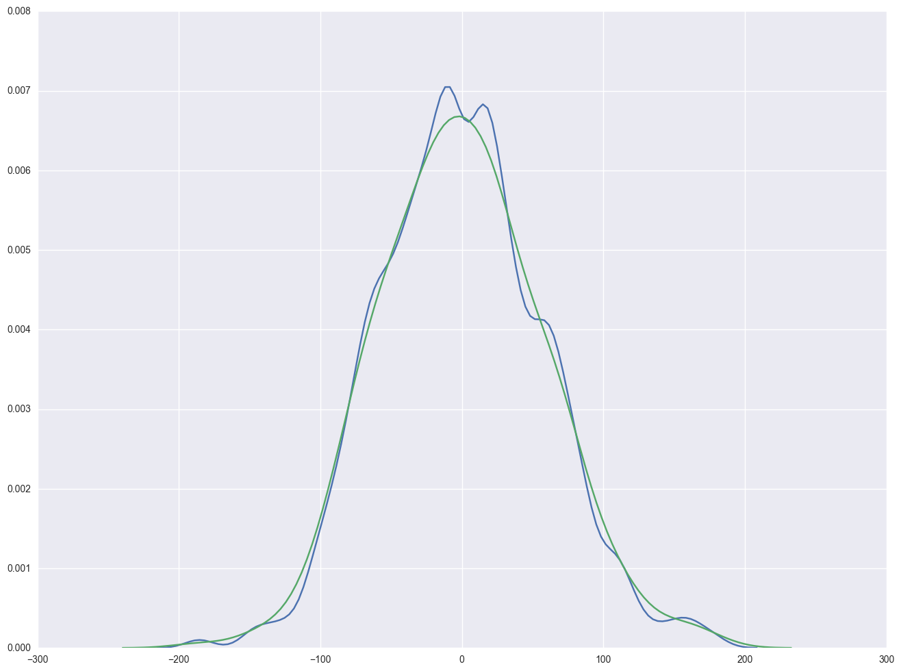
sns.kdeplot(np.array(elem1res.resid), bw=10)
sns.distplot(np.array(elem1res.resid), hist=False)
<matplotlib.axes._subplots.AxesSubplot at 0x23bc05c0>
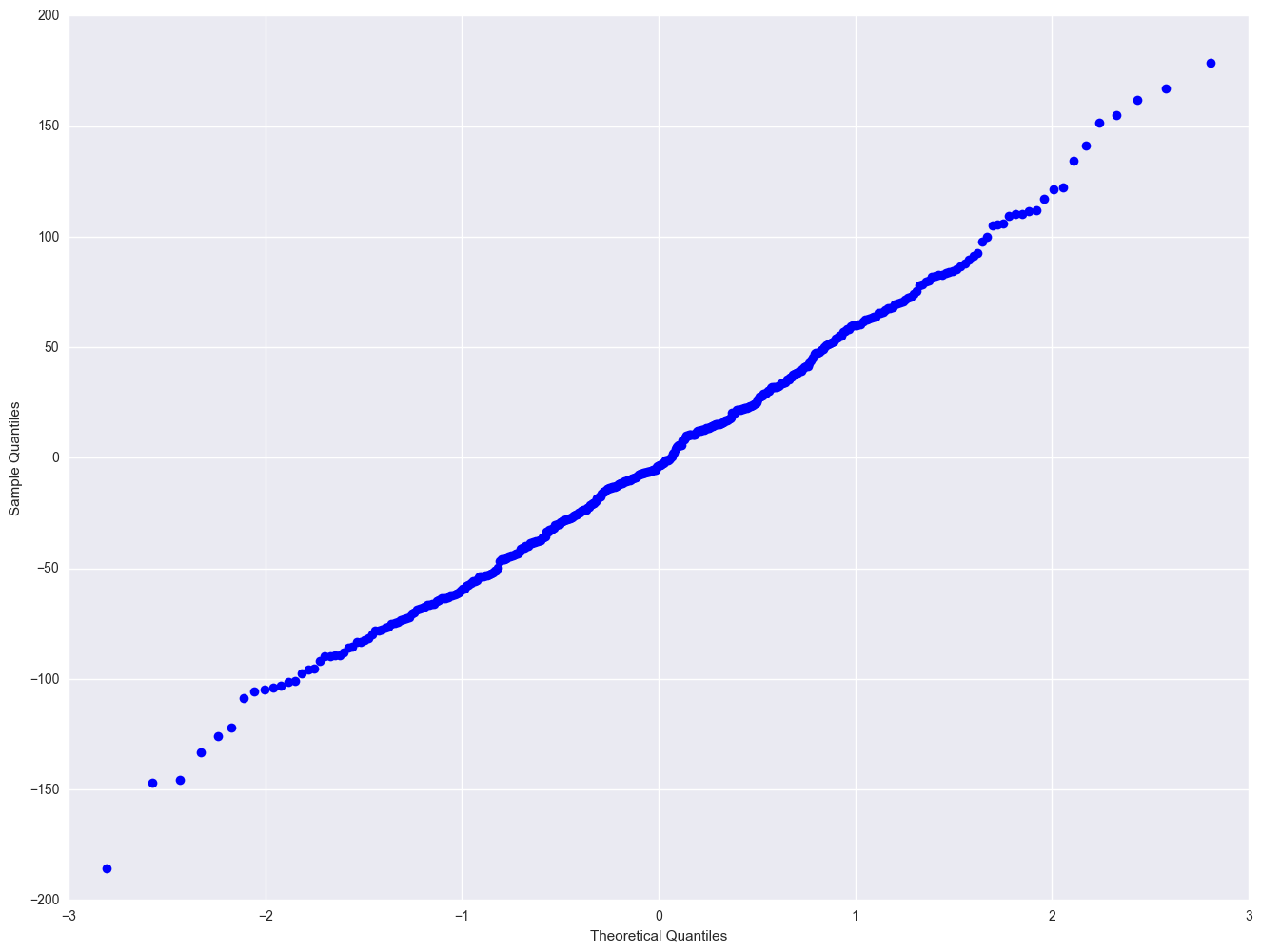
sm.qqplot(elem1res.resid)
plt.show()
import pylab
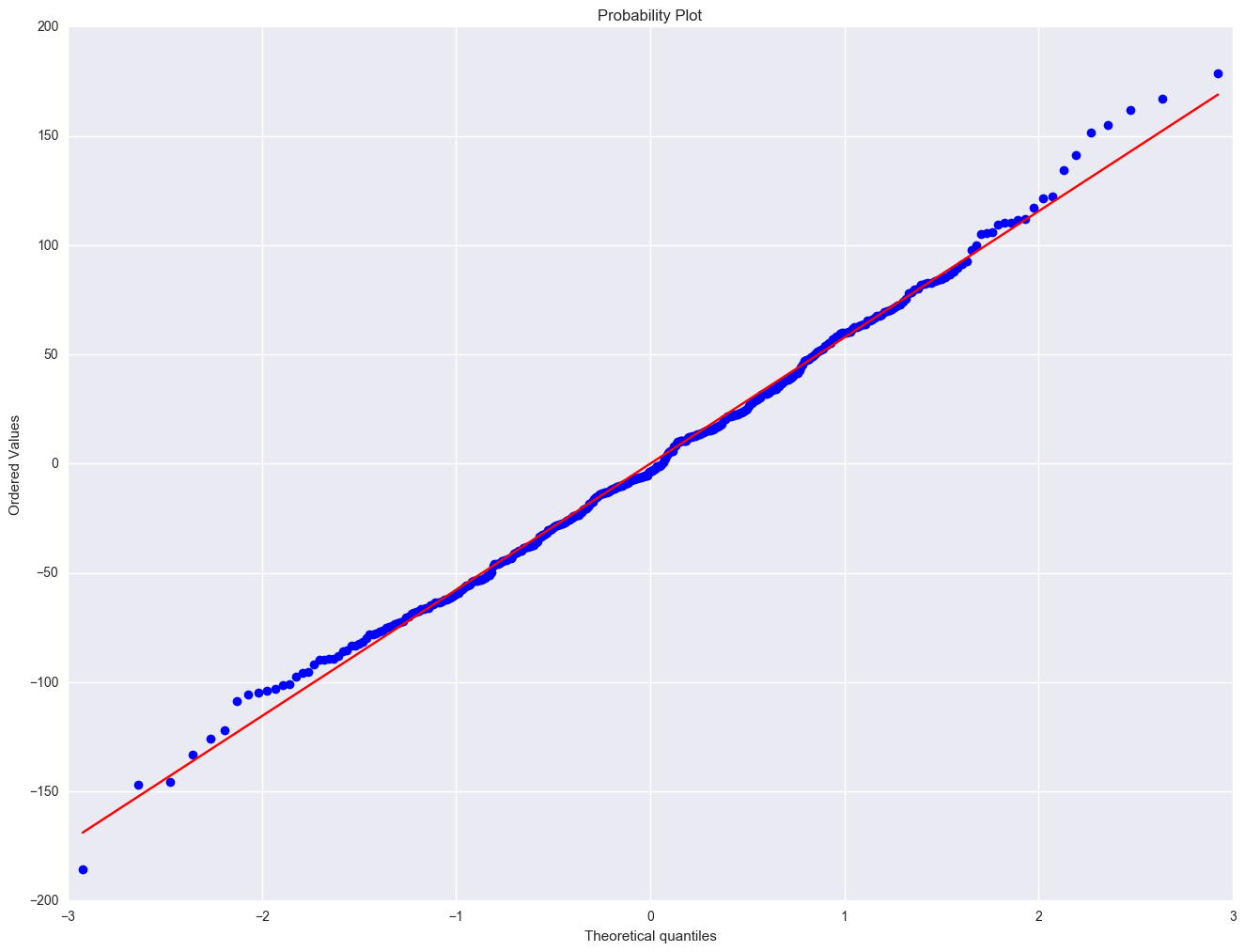
scipystats.probplot(elem1res.resid, dist="norm", plot=pylab)
pylab.show()
'''
by default, scipy stats.kstest for normal will assume mean 0 and stdev 1. To use this, the data should be normalized first
'''
resid = elem1res.resid
norm_resid = (elem1res.resid - np.mean(elem1res.resid)) / np.std(elem1res.resid)
print scipystats.kstest(norm_resid, 'norm')

# or use the statsmodels provided function kstest_normal to use kolmogorov-smirnov test or Anderson-Darling test
print stats.diagnostic.kstest_normal(elem1res.resid, pvalmethod='approx')
print stats.diagnostic.normal_ad(elem1res.resid)
KstestResult(statistic=0.032723261818185578, pvalue=0.78506446901572213)
(0.032676218847940308, 0.35190400492542645)
(0.34071240334691311, 0.49471893268937844)
Severe outliers consist of those points that are either 3 inter-quartile-ranges below the first quartile or 3 inter-quartile-ranges above the third quartile. The presence of any severe outliers should be sufficient evidence to reject normality at a 5% significance level. Mild outliers are common in samples of any size. In our case, we don't have any severe outliers and the distribution seems fairly symmetric. The residuals have an approximately normal distribution. (See the output of the proc univariate above.)
In the Kilmogorov-Smirnov test or Anderson-Darling test for normality, the p-value is based on the assumption that the distribution is normal. In our example, the p-value is very large, indicating that we cannot reject that residuals is normally distributed.
2.3 Tests for Heteroscedasticity
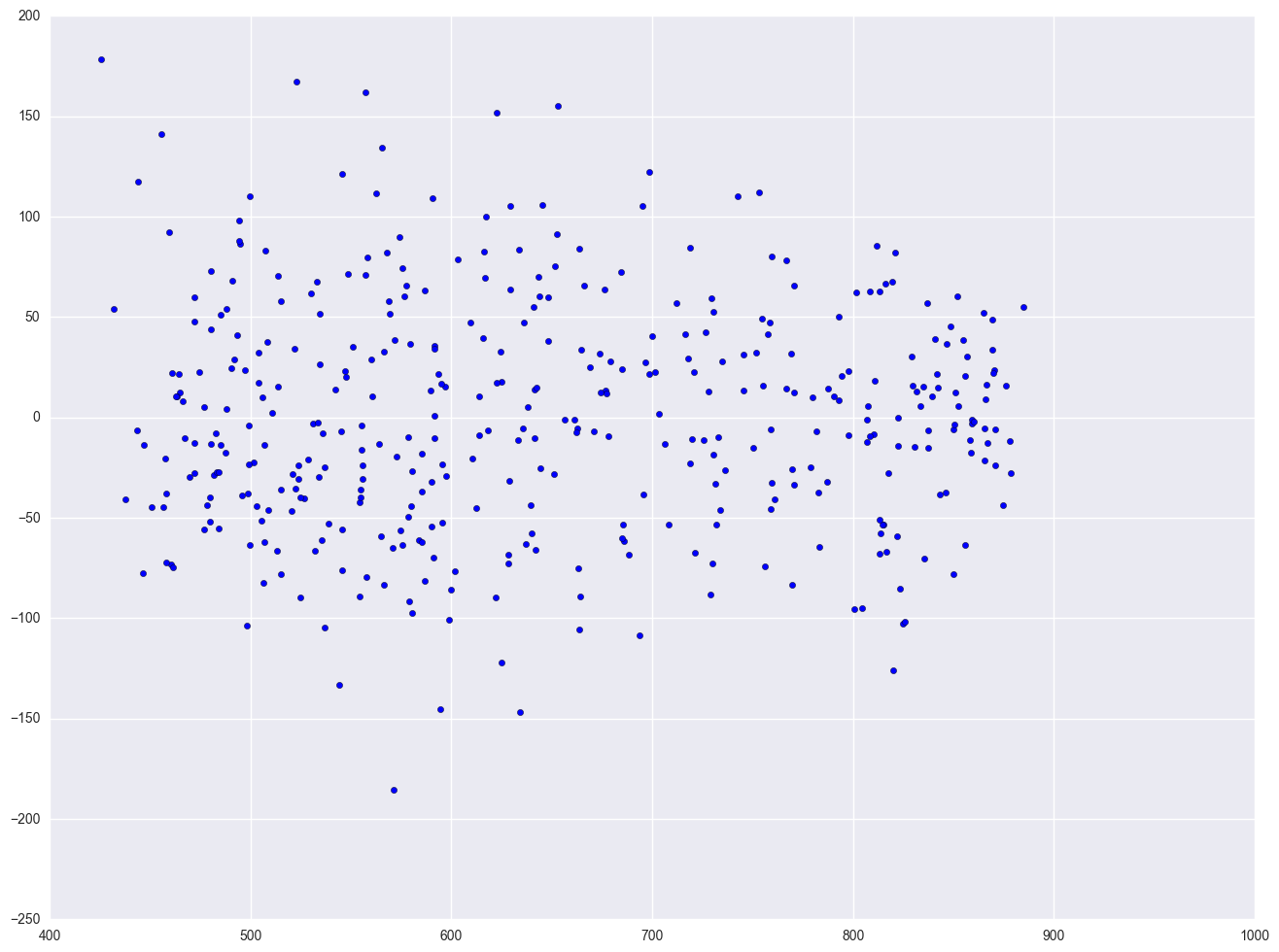
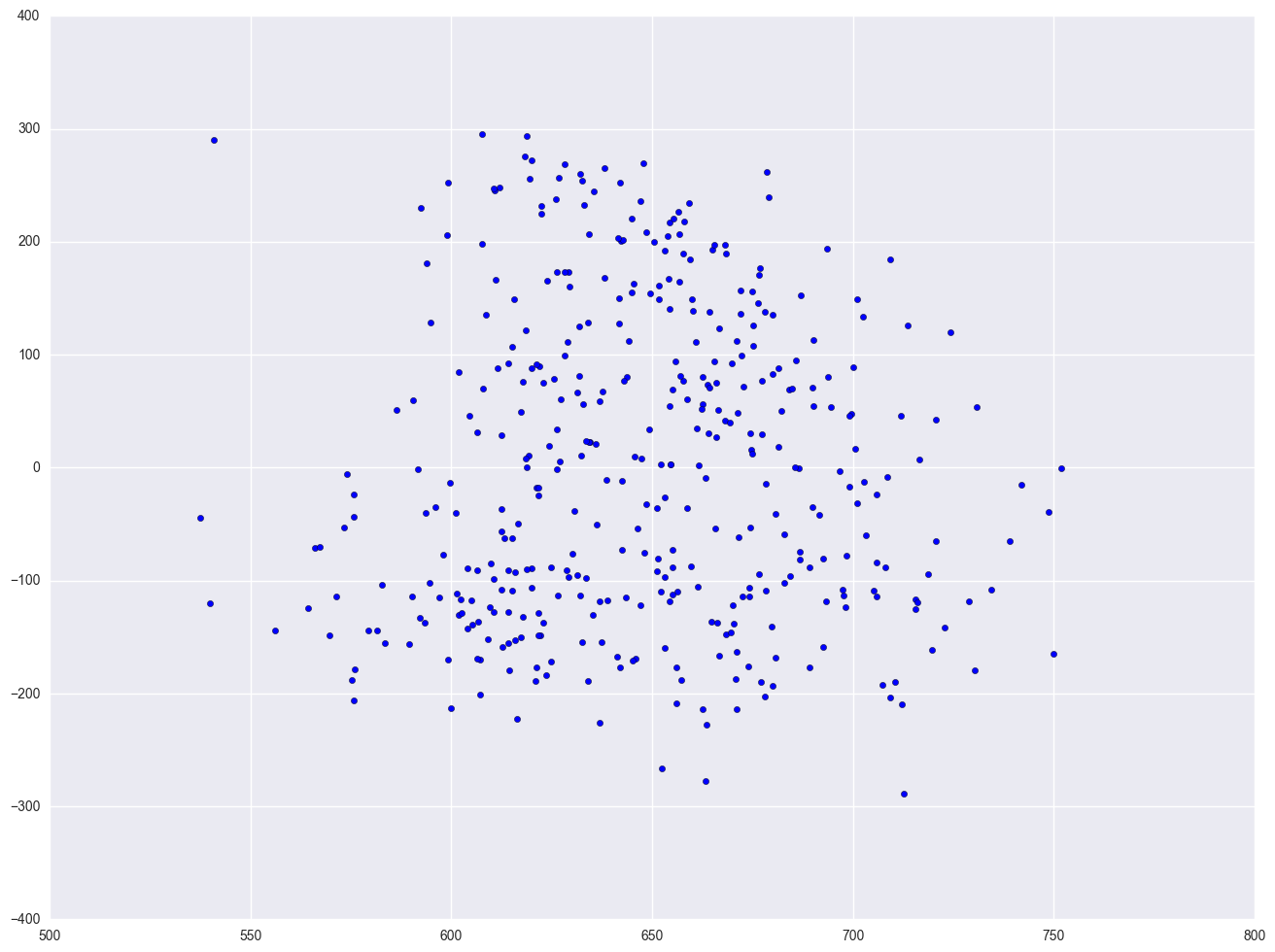
One of the main assumptions for the ordinary least squares regression is the homogeneity of variance of the residuals. If the model is well-fitted, there should be no pattern to the residuals plotted against the fitted values. If the variance of the residuals is non-constant, then the residual variance is said to be "heteroscedastic." There are graphical and non-graphical methods for detecting heteroscedasticity. A commonly used graphical method is to plot the residuals versus fitted (predicted) values. We see that the pattern of the data points is getting a little narrower towards the right end, which is an indication of mild heteroscedasticity.
lm = smf.ols(formula = "api00 ~ meals + ell + emer", data = elemapi2).fit()

resid = lm.resid
plt.scatter(lm.predict(), resid)
<matplotlib.collections.PathCollection at 0x261445f8>
# p-value here is different from SAS output, need double check
stats.diagnostic.het_white(resid, lm.model.exog, retres = False)
(18.352755736667305,
 0.031294634010796941,
 2.0838250344433504,
 0.029987789753355969)
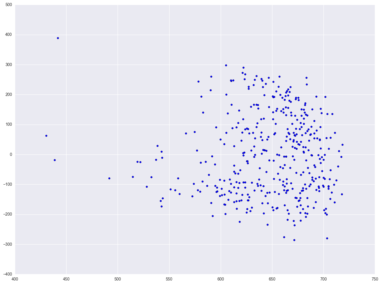
lm2 = smf.ols(formula = "api00 ~ enroll", data = elemapi2).fit()

plt.scatter(lm2.predict(), lm2.resid)
<matplotlib.collections.PathCollection at 0x25ccb470>
elemapi2['log_enroll'] = elemapi2.enroll.map(lambda x: math.log(x))
lm3 = smf.ols(formula = "api00 ~ log_enroll", data = elemapi2).fit()

plt.scatter(lm3.predict(), lm3.resid)
<matplotlib.collections.PathCollection at 0x28a10a20>
Finally, let's revisit the model we used at the start of this section, predicting api00 from meals, ell and emer. Using this model, the distribution of the residuals looked very nice and even across the fitted values. What if we add enroll to this model? Will this automatically ruin the distribution of the residuals? Let's add it and see.
lm4 = smf.ols(formula = "api00 ~ meals + ell + emer + enroll", data = elemapi2).fit()

resid = lm4.resid
plt.scatter(lm4.predict(), resid)
<matplotlib.collections.PathCollection at 0x28b71828>
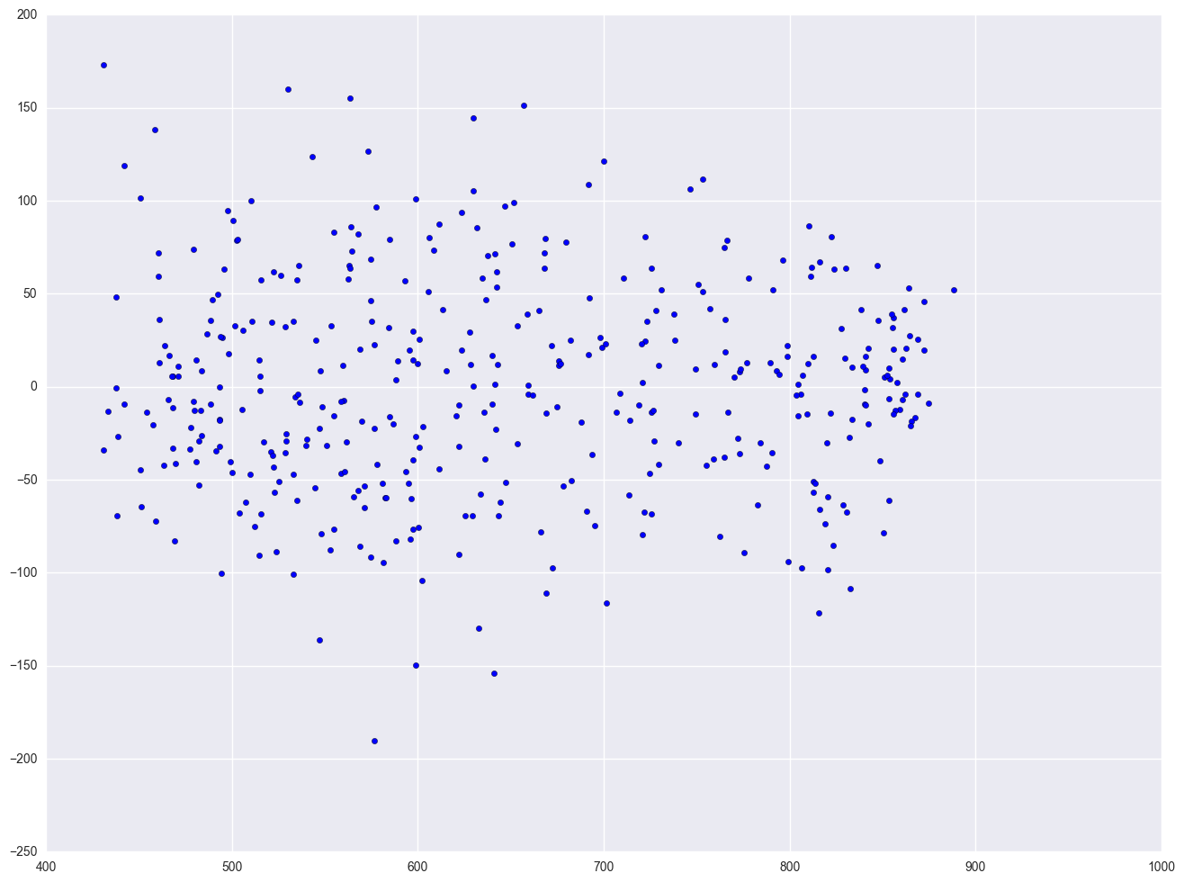
As you can see, the distribution of the residuals looks fine, even after we added the variable enroll. When we had just the variable enroll in the model, we did a log transformation to improve the distribution of the residuals, but when enroll was part of a model with other variables, the residuals looked good enough so that no transformation was needed. This illustrates how the distribution of the residuals, not the distribution of the predictor, was the guiding factor in determining whether a transformation was needed.
2.4 Tests for Collinearity
When there is a perfect linear relationship among the predictors, the estimates for a regression model cannot be uniquely computed. The term collinearity describes two variables are near perfect linear combinations of one another. When more than two variables are involved, it is often called multicollinearity, although the two terms are often used interchangeably.
The primary concern is that as the degree of multicollinearity increases, the regression model estimates of the coefficients become unstable and the standard errors for the coefficients can get wildly inflated. In this section, we will explore some SAS options used with the model statement that help to detect multicollinearity.
We can use the vif option to check for multicollinearity. vif stands for variance inflation factor. As a rule of thumb, a variable whose VIF values is greater than 10 may merit further investigation. Tolerance, defined as 1/VIF, is used by many researchers to check on the degree of collinearity. A tolerance value lower than 0.1 is comparable to a VIF of 10. It means that the variable could be considered as a linear combination of other independent variables. The tol option on the model statement gives us these values. Let's first look at the regression we did from the last section, the regression model predicting api00 from meals, ell and emer, and use the vif and tol options with the model statement.
from patsy import dmatrices
from statsmodels.stats.outliers_influence import variance_inflation_factor

lm = smf.ols(formula = "api00 ~ meals + ell + emer", data = elemapi2).fit()
y, X = dmatrices("api00 ~ meals + ell + emer", data = elemapi2, return_type = "dataframe")
vif = [variance_inflation_factor(X.values, i) for i in range(X.shape[1])]
print vif
[4.6883371380582997, 2.7250555232887432, 2.5105120172587836, 1.4148169984086651]
We know the multicollinearity is caused the high correlation between the indepentent variables. So let's check the correlation between the vatiables. First we need to drop the added constant column which are all equal to 1. Then np.corrcoef or df.corr will calculate the correlation coefficient. We can also calculate the eigen value and eigen vectors of the correlation matrix to check the details.
corr = np.corrcoef(X.drop("Intercept", axis = 1), rowvar = 0)
print "correlation from np.corrcoef is "
print corr

print '\n'
print "correlation from df.corr() is "
print X.drop("Intercept", axis = 1).corr()

print '\n'

w, v = np.linalg.eig(corr)
print "the eigen value of the correlation coefficient is "
print w
correlation from np.corrcoef is
[[ 1.          0.77237718  0.53303874]
 [ 0.77237718  1.          0.47217948]
 [ 0.53303874  0.47217948  1.        ]]


correlation from df.corr() is
          meals       ell      emer
meals  1.000000  0.772377  0.533039
ell    0.772377  1.000000  0.472179
emer   0.533039  0.472179  1.000000


the eigen value of the correlation coefficient is
[ 2.19536815  0.22351013  0.58112172]
2.5 Tests on Nonlinearity
When we do linear regression, we assume that the relationship between the response variable and the predictors is linear. This is the assumption of linearity. If this assumption is violated, the linear regression will try to fit a straight line to data that does not follow a straight line. Checking the linear assumption in the case of simple regression is straightforward, since we only have one predictor. All we have to do is a scatter plot between the response variable and the predictor to see if nonlinearity is present, such as a curved band or a big wave-shaped curve. For example, let us use a data file called nations.sav that has data about a number of nations around the world.
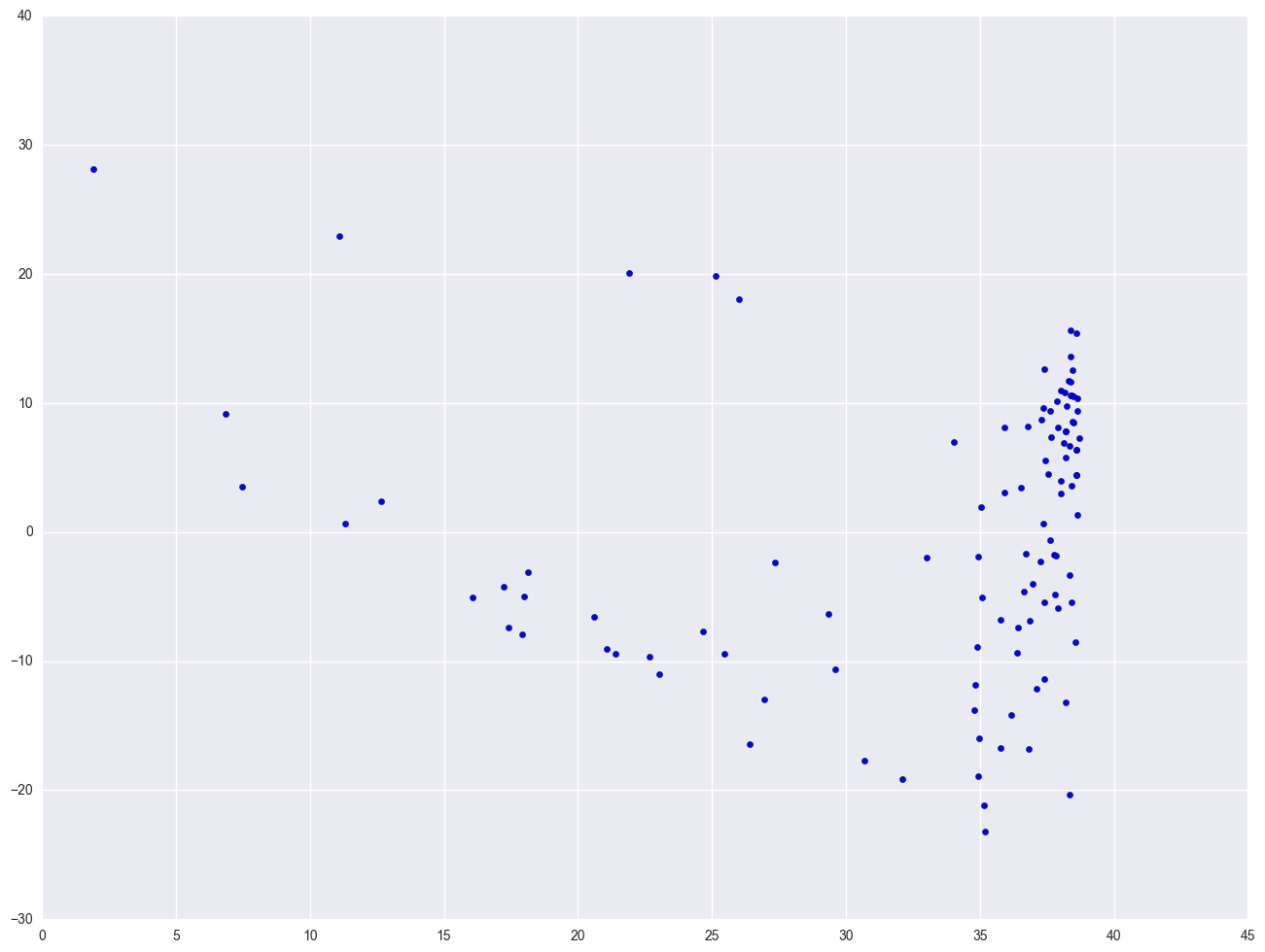
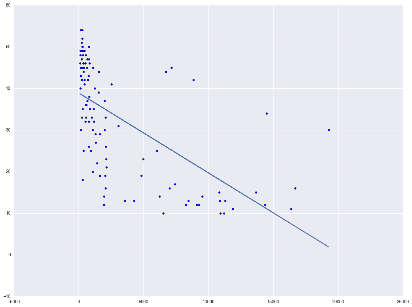
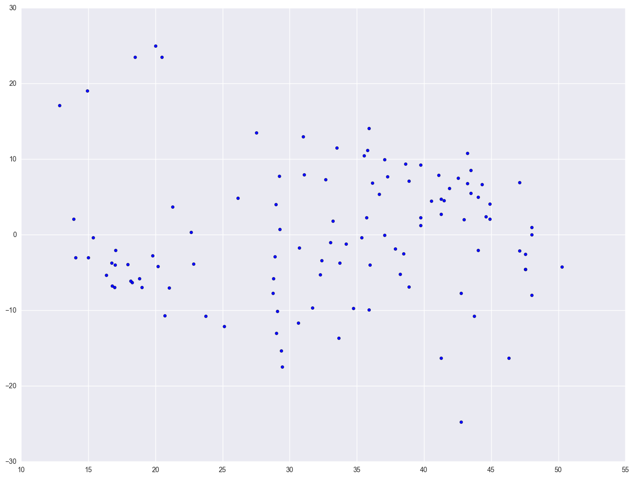
Let's look at the relationship between GNP per capita (gnpcap) and births (birth). Below if we look at the scatterplot between gnpcap and birth, we can see that the relationship between these two variables is quite non-linear. We added a regression line to the chart, and you can see how poorly the line fits this data. Also, if we look at the residuals by predicted plot, we see that the residuals are not nearly homoscedastic, due to the non-linearity in the relationship between gnpcap and birth.
nations = pd.read_csv(mypath + "nations.csv")
# print nations.describe()

lm = smf.ols(formula = "birth ~ gnpcap", data = nations).fit()
print lm.summary()

plt.scatter(lm.predict(), lm.resid)
plt.show()

plt.scatter(nations.gnpcap, nations.birth)
plt.plot(nations.gnpcap, lm.params[0] + lm.params[1] * nations.gnpcap, '-')
plt.show()
                            OLS Regression Results
==============================================================================
Dep. Variable:                  birth   R-squared:                       0.392
Model:                            OLS   Adj. R-squared:                  0.387
Method:                 Least Squares   F-statistic:                     69.05
Date:                Mon, 26 Dec 2016   Prob (F-statistic):           3.27e-13
Time:                        15:42:45   Log-Likelihood:                -411.80
No. Observations:                 109   AIC:                             827.6
Df Residuals:                     107   BIC:                             833.0
Df Model:                           1
Covariance Type:            nonrobust
==============================================================================
                 coef    std err          t      P>|t|      [95.0% Conf. Int.]
------------------------------------------------------------------------------
Intercept     38.9242      1.261     30.856      0.000        36.423    41.425
gnpcap        -0.0019      0.000     -8.309      0.000        -0.002    -0.001
==============================================================================
Omnibus:                        1.735   Durbin-Watson:                   1.824
Prob(Omnibus):                  0.420   Jarque-Bera (JB):                1.335
Skew:                          -0.011   Prob(JB):                        0.513
Kurtosis:                       2.458   Cond. No.                     6.73e+03
==============================================================================

Warnings:
[1] Standard Errors assume that the covariance matrix of the errors is correctly specified.
[2] The condition number is large, 6.73e+03. This might indicate that there are
strong multicollinearity or other numerical problems.
Now we are going to modify the above scatterplot by adding a lowess (also called "loess") smoothing line. We show only the graph with the 0.4 smooth.
from statsmodels.nonparametric.smoothers_lowess import lowess
lowess_df = pd.DataFrame(lowess(endog = nations.birth, exog = nations.gnpcap, frac = 0.4), columns = ["gnpcap", "birth"])

plt.plot(lowess_df.gnpcap, lowess_df.birth)
plt.scatter(nations.gnpcap, nations.birth)
plt.plot(nations.gnpcap, lm.params[0] + lm.params[1] * nations.gnpcap, '-')
plt.xlabel("transform of gnpcap")
plt.ylabel("transform of birth")
plt.show()
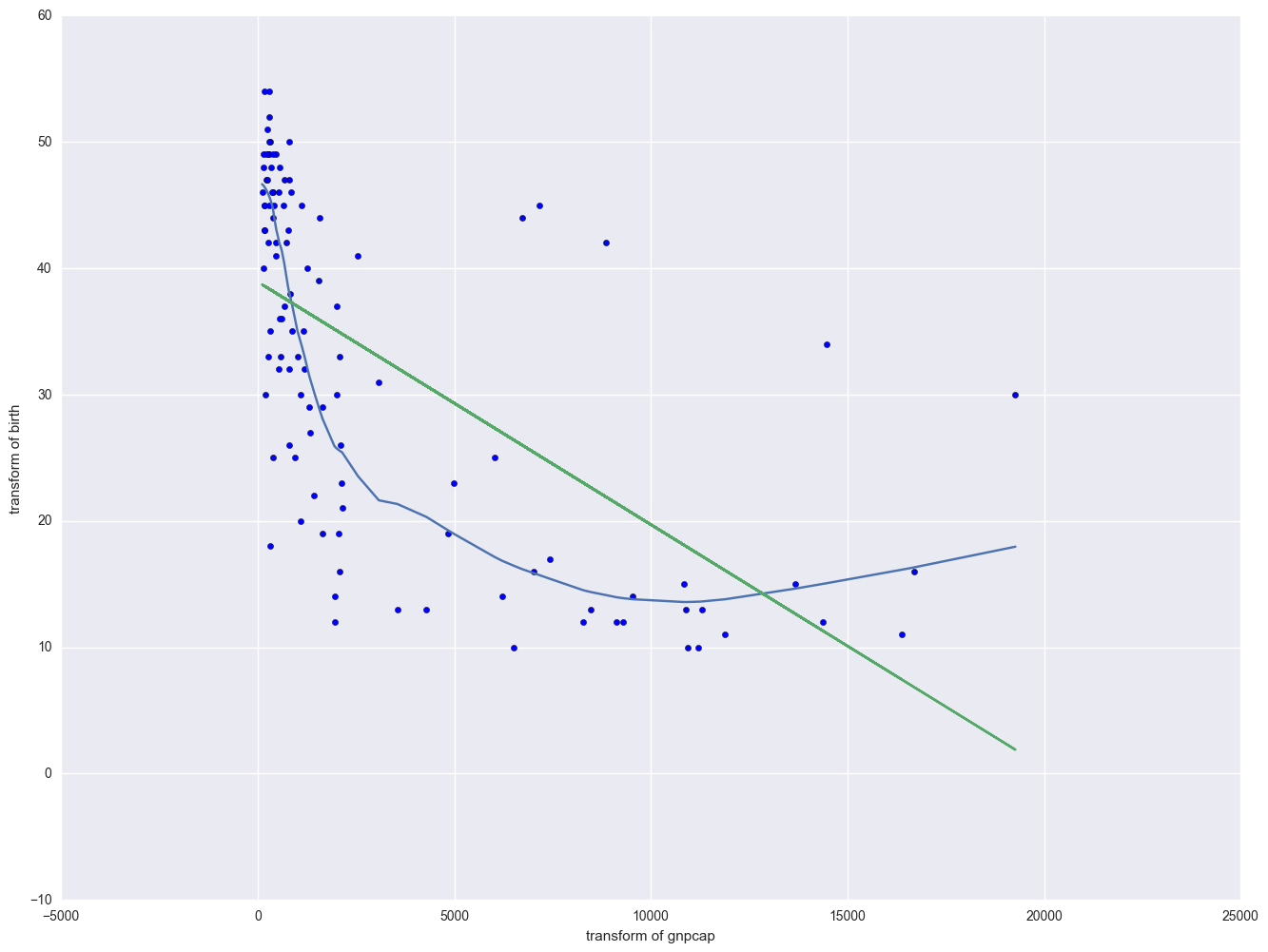
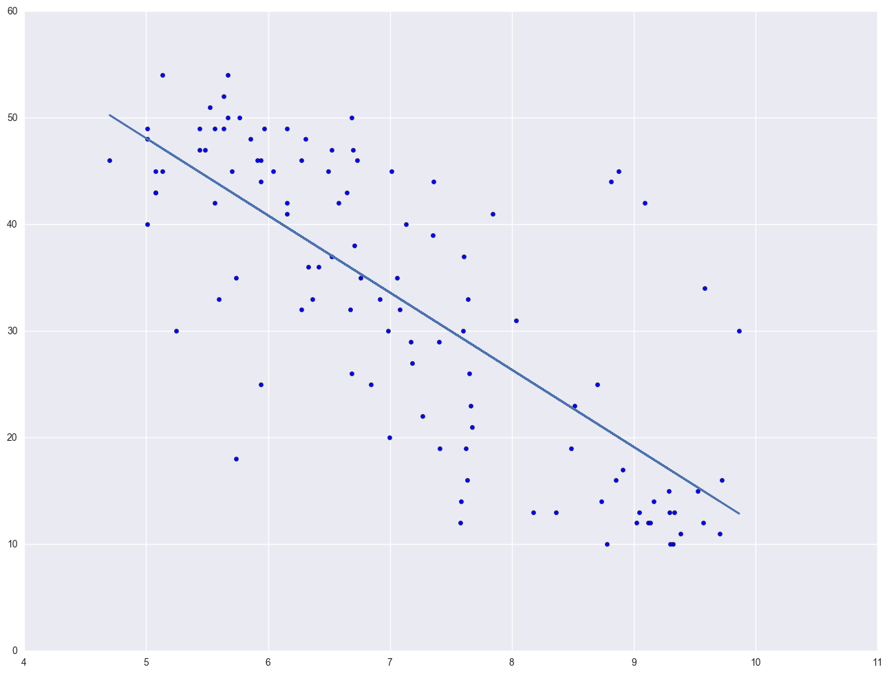
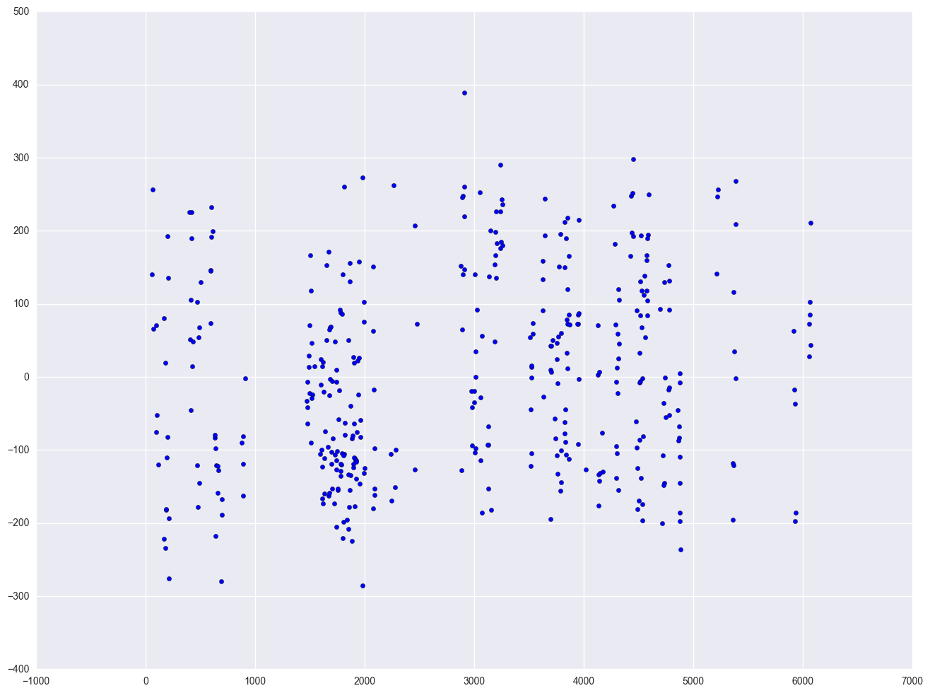
The lowess line fits much better than the OLS linear regression. In trying to see how to remedy these, we notice that the gnpcap scores are quite skewed with most values being near 0, and a handful of values of 10,000 and higher. This suggests to us that some transformation of the variable may be useful. One of the commonly used transformations is a log transformation. Let's try it below. As you see, the scatterplot between lgnpcap and birth looks much better with the regression line going through the heart of the data. Also, the plot of the residuals by predicted values look much more reasonable.
nations["log_gnpcap"] = nations.gnpcap.map(lambda x: math.log(x))
lm2 = smf.ols("birth ~ log_gnpcap", data = nations).fit()
print lm2.summary()

plt.scatter(lm2.predict(), lm2.resid)
plt.show()

plt.scatter(nations.log_gnpcap, nations.birth)
plt.plot(nations.log_gnpcap, lm2.params[0] + lm2.params[1] * nations.log_gnpcap, '-')
plt.show()
                            OLS Regression Results
==============================================================================
Dep. Variable:                  birth   R-squared:                       0.571
Model:                            OLS   Adj. R-squared:                  0.567
Method:                 Least Squares   F-statistic:                     142.6
Date:                Mon, 26 Dec 2016   Prob (F-statistic):           2.12e-21
Time:                        16:08:02   Log-Likelihood:                -392.77
No. Observations:                 109   AIC:                             789.5
Df Residuals:                     107   BIC:                             794.9
Df Model:                           1
Covariance Type:            nonrobust
==============================================================================
                 coef    std err          t      P>|t|      [95.0% Conf. Int.]
------------------------------------------------------------------------------
Intercept     84.2773      4.397     19.168      0.000        75.561    92.993
log_gnpcap    -7.2385      0.606    -11.941      0.000        -8.440    -6.037
==============================================================================
Omnibus:                        2.875   Durbin-Watson:                   1.790
Prob(Omnibus):                  0.237   Jarque-Bera (JB):                2.267
Skew:                           0.282   Prob(JB):                        0.322
Kurtosis:                       3.425   Cond. No.                         37.8
==============================================================================

Warnings:
[1] Standard Errors assume that the covariance matrix of the errors is correctly specified.
This section has shown how you can use scatterplots to diagnose problems of non-linearity, both by looking at the scatterplots of the predictor and outcome variable, as well as by examining the residuals by predicted values. These examples have focused on simple regression; however, similar techniques would be useful in multiple regression. However, when using multiple regression, it would be more useful to examine partial regression plots instead of the simple scatterplots between the predictor variables and the outcome variable.
2.6 Model Specification
A model specification error can occur when one or more relevant variables are omitted from the model or one or more irrelevant variables are included in the model. If relevant variables are omitted from the model, the common variance they share with included variables may be wrongly attributed to those variables, and the error term is inflated. On the other hand, if irrelevant variables are included in the model, the common variance they share with included variables may be wrongly attributed to them. Model specification errors can substantially affect the estimate of regression coefficients.
Consider the model below. This regression suggests that as class size increases the academic performance increases. Before we publish results saying that increased class size is associated with higher academic performance, let's check the model specification.
elemapi2_0 = elemapi2[~np.isnan(elemapi2.acs_k3)]
lm = smf.ols("api00 ~ acs_k3", data = elemapi2_0).fit()
elemapi2_0.loc[:, "fv"] = lm.predict()
elemapi2_0.loc[:, "fvsquare"] = elemapi2_0.fv ** 2
There are a couple of methods to detect specification errors. A link test performs a model specification test for single-equation models. It is based on the idea that if a regression is properly specified, one should not be able to find any additional independent variables that are significant except by chance. To conduct this test, you need to obtain the fitted values from your regression and the squares of those values. The model is then refit using these two variables as predictors. The fitted value should be significant because it is the predicted value. One the other hand, the fitted values squared shouldn't be significant, because if our model is specified correctly, the squared predictions should not have much of explanatory power. That is, we wouldn't expect the fitted value squared to be a significant predictor if our model is specified correctly. So we will be looking at the p-value for the fitted value squared.
lm = smf.ols("api00 ~ fv + fvsquare", data = elemapi2_0).fit()
print lm.summary()
                            OLS Regression Results
==============================================================================
Dep. Variable:                  api00   R-squared:                       0.035
Model:                            OLS   Adj. R-squared:                  0.030
Method:                 Least Squares   F-statistic:                     7.089
Date:                Tue, 27 Dec 2016   Prob (F-statistic):           0.000944
Time:                        14:52:59   Log-Likelihood:                -2529.9
No. Observations:                 398   AIC:                             5066.
Df Residuals:                     395   BIC:                             5078.
Df Model:                           2
Covariance Type:            nonrobust
==============================================================================
                 coef    std err          t      P>|t|      [95.0% Conf. Int.]
------------------------------------------------------------------------------
Intercept   3884.5065   2617.696      1.484      0.139     -1261.853  9030.866
fv           -11.0501      8.105     -1.363      0.174       -26.984     4.883
fvsquare       0.0093      0.006      1.488      0.138        -0.003     0.022
==============================================================================
Omnibus:                      135.464   Durbin-Watson:                   1.420
Prob(Omnibus):                  0.000   Jarque-Bera (JB):               20.532
Skew:                           0.048   Prob(JB):                     3.48e-05
Kurtosis:                       1.891   Cond. No.                     1.58e+08
==============================================================================

Warnings:
[1] Standard Errors assume that the covariance matrix of the errors is correctly specified.
[2] The condition number is large, 1.58e+08. This might indicate that there are
strong multicollinearity or other numerical problems.
Let's try adding one more variable, meals, to the above model and then run the link test again.
lm = smf.ols("api00 ~ acs_k3 + full + fv", data = elemapi2_0).fit()
print lm.summary()
                            OLS Regression Results
==============================================================================
Dep. Variable:                  api00   R-squared:                       0.339
Model:                            OLS   Adj. R-squared:                  0.335
Method:                 Least Squares   F-statistic:                     101.2
Date:                Tue, 27 Dec 2016   Prob (F-statistic):           3.29e-36
Time:                        14:54:29   Log-Likelihood:                -2454.6
No. Observations:                 398   AIC:                             4915.
Df Residuals:                     395   BIC:                             4927.
Df Model:                           2
Covariance Type:            nonrobust
==============================================================================
                 coef    std err          t      P>|t|      [95.0% Conf. Int.]
------------------------------------------------------------------------------
Intercept     -0.3727      0.515     -0.724      0.469        -1.384     0.639
acs_k3         6.4796      8.922      0.726      0.468       -11.060    24.020
full           5.3898      0.396     13.598      0.000         4.611     6.169
fv             0.1057      0.271      0.390      0.697        -0.427     0.639
==============================================================================
Omnibus:                       15.537   Durbin-Watson:                   1.367
Prob(Omnibus):                  0.000   Jarque-Bera (JB):                7.217
Skew:                          -0.017   Prob(JB):                       0.0271
Kurtosis:                       2.341   Cond. No.                     9.77e+17
==============================================================================

Warnings:
[1] Standard Errors assume that the covariance matrix of the errors is correctly specified.
[2] The smallest eigenvalue is 1.79e-28. This might indicate that there are
strong multicollinearity problems or that the design matrix is singular.
The link test is once again non-significant. Note that after including meals and full, the coefficient for class size is no longer significant. While acs_k3 does have a positive relationship with api00 when no other variables are in the model, when we include, and hence control for, other important variables, acs_k3 is no longer significantly related to api00 and its relationship to api00 is no longer positive.
2.7 Issues of Independence
The statement of this assumption is that the errors associated with one observation are not correlated with the errors of any other observation cover several different situations. Consider the case of collecting data from students in eight different elementary schools. It is likely that the students within each school will tend to be more like one another that students from different schools, that is, their errors are not independent. We will deal with this type of situation in Chapter 4.
Another way in which the assumption of independence can be broken is when data are collected on the same variables over time. Let's say that we collect truancy data every semester for 12 years. In this situation it is likely that the errors for observation between adjacent semesters will be more highly correlated than for observations more separated in time. This is known as autocorrelation. When you have data that can be considered to be time-series, you should use the dw option that performs a Durbin-Watson test for correlated residuals.
We don't have any time-series data, so we will use the elemapi2 dataset and pretend that snum indicates the time at which the data were collected. We will sort the data on snum to order the data according to our fake time variable and then we can run the regression analysis with the dw option to request the Durbin-Watson test. The Durbin-Watson statistic has a range from 0 to 4 with a midpoint of 2. The observed value in our example is less than 2, which is not surprising since our data are not truly time-series.
lm = smf.ols(formula = "api00 ~ enroll", data = elemapi2).fit()
print lm.summary()
print "Durbin-Watson test statistics is " + str(stools.durbin_watson(lm.resid))

plt.scatter(elemapi2.snum, lm.resid)
plt.show()
                            OLS Regression Results
==============================================================================
Dep. Variable:                  api00   R-squared:                       0.101
Model:                            OLS   Adj. R-squared:                  0.099
Method:                 Least Squares   F-statistic:                     44.83
Date:                Tue, 27 Dec 2016   Prob (F-statistic):           7.34e-11
Time:                        15:00:28   Log-Likelihood:                -2528.8
No. Observations:                 400   AIC:                             5062.
Df Residuals:                     398   BIC:                             5070.
Df Model:                           1
Covariance Type:            nonrobust
==============================================================================
                 coef    std err          t      P>|t|      [95.0% Conf. Int.]
------------------------------------------------------------------------------
Intercept    744.2514     15.933     46.711      0.000       712.928   775.575
enroll        -0.1999      0.030     -6.695      0.000        -0.259    -0.141
==============================================================================
Omnibus:                       43.040   Durbin-Watson:                   1.342
Prob(Omnibus):                  0.000   Jarque-Bera (JB):               17.113
Skew:                           0.277   Prob(JB):                     0.000192
Kurtosis:                       2.152   Cond. No.                     1.26e+03
==============================================================================

Warnings:
[1] Standard Errors assume that the covariance matrix of the errors is correctly specified.
[2] The condition number is large, 1.26e+03. This might indicate that there are
strong multicollinearity or other numerical problems.
Durbin-Watson test statistics is 1.34234658795
2.8 Summary
In this chapter, we have used a number of tools in SAS for determining whether our data meets the regression assumptions. Below, we list the major commands we demonstrated organized according to the assumption the command was shown to test.
Detecting Unusual and Influential Data
    scatterplots of the dependent variables versus the independent variable
    looking at the largest values of the studentized residuals, leverage, Cook's D, DFFITS and DFBETAs

Tests for Normality of Residuals Tests for Heteroscedasity
    kernel density plot
    quantile-quantile plots
    standardized normal probability plots
    Shapiro-Wilk W test
    scatterplot of residuals versus predicted (fitted) values
    White test

Tests for Multicollinearity
    looking at VIF
    looking at tolerance

Tests for Non-Linearity
    scatterplot of independent variable versus dependent variable

Tests for Model Specification
    time series
    Durbin-Watson test
reference
- Interpreting plot.lm()
- statsmodels.stats.outliers_influence.OLSInfluence
- Regression Diagnostics and Specification Tests
- Statistics stats
- lowess smoothing
- outlier influence
from statsmodels.stats.outliers_influence import OLSInfluence
print pd.Series(OLSInfluence(lm).influence, name = "Leverage")