The data is time-varying value for each instrument. Each instrument has id, and timestamp. y is the response value to be predicted. All the others are the anonymized features.
0. Introduction
This dataset contains anonymized features pertaining to a time-varying value for a financial instrument. Each instrument has an id. Time is represented by the 'timestamp' feature and the variable to predict is 'y'. No further information will be provided on the meaning of the features, the transformations that were applied to them, the timescale, or the type of instruments that are included in the data. Moreover, in accordance with competition rules, participants must not use data other than the data linked from the competition website for the purpose of use in this competition to develop and test their models and submissions.
import numpy as np
import pandas as pd
import seaborn as sns
import matplotlib.pyplot as plt

%matplotlib inline
plt.figure(figsize=(16, 12))
df = pd.read_hdf(r'../input/train.h5')
1. data description
First we will have a look how many columns are there in the data, what are the columns. How many data are there totally, How many isstrements are there(unique id), and how many timestamp observed for each instrement.
df.columns
Index([u'id', u'timestamp', u'derived_0', u'derived_1', u'derived_2',
       u'derived_3', u'derived_4', u'fundamental_0', u'fundamental_1',
       u'fundamental_2',
       ...
       u'technical_36', u'technical_37', u'technical_38', u'technical_39',
       u'technical_40', u'technical_41', u'technical_42', u'technical_43',
       u'technical_44', u'y'],
      dtype='object', length=111)
it is like the columns are fake names. it tells us 5 are derived, 63 are fundamental, ant 40 are techinical.
cols = pd.Series(df.columns.map(lambda x: x[:8])).value_counts().values.tolist()
print("Fundmental columns: {}, Techinical columns: {}, Derived columns: {}".format(*cols))
Fundmental columns: 63, Techinical columns: 40, Derived columns: 5
There are 1424 unique instrument id. Each id has unique timestamps. The instruments like id=1229, 1893 only has two timestamps. The instruments id = 1066, 704 have 1813 timestamps.
print len(df.id.unique())
print df.groupby('id').size().sort_values().head()
print df.groupby('id').size().sort_values(ascending = False).head()
1424
id
1229     2
1893     2
435      2
1056     8
980     12
dtype: int64
id
1066    1813
704     1813
697     1813
699     1813
1548    1813
dtype: int64
1.1. check the missing data
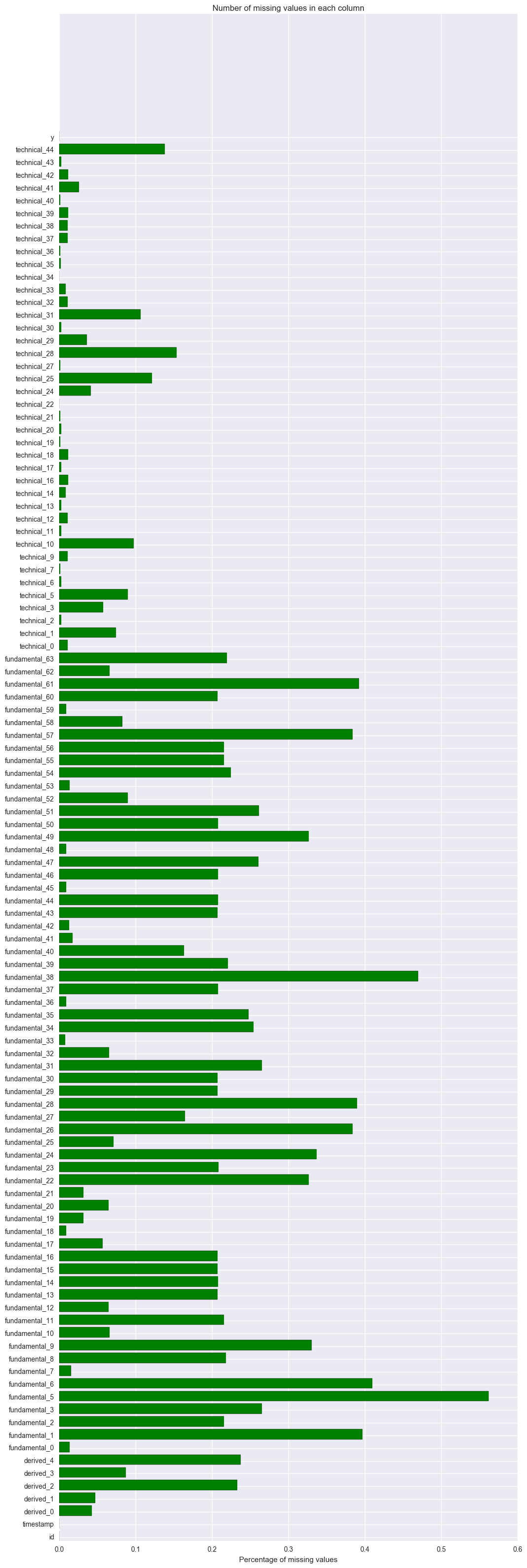
Col 3 to col 110 are the independent variables. Most of these columns have missing values. The following is to count how many missing values are there for each variable and the percentage of missing values. The top 5 variables having the most missing values are fundamental_5 (56%), fundamental_38(47%), fundamental_6(41%), fundamental_1(40%) and fundamental_61(39%).
So we need to impute missing values. shall we impute directly or shall we impute within each group by id, timestamp or id+timestamp?
missing_cnts = df.isnull().sum(axis = 0)
missing_pct = missing_cnts / df.shape[0]
missing_pct.sort_values(ascending = False).head()
fundamental_5     0.562336
fundamental_38    0.469669
fundamental_6     0.410126
fundamental_1     0.396941
fundamental_61    0.392692
dtype: float64
ind = np.arange(df.shape[1])
width = 0.6
fig, ax = plt.subplots(figsize=(12,40))
rects = ax.barh(ind, missing_pct.values, color='g')
ax.set_yticks(ind+((width)/2.))
ax.set_yticklabels(missing_cnts.index, rotation='horizontal')
ax.set_xlabel("Percentage of missing values")
ax.set_title("Number of missing values in each column")
plt.show()
1.2. y variable
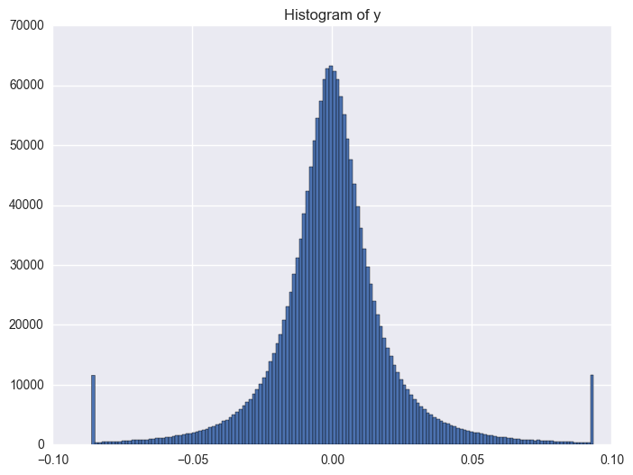
y distribution is like normal distribution, except that there are two high tails. We need to have a look why there are ourliers on the tail around 0.0934 and -0.086. It shows the data bas been capped and floored.
Then the questions comes: how shall we deal with the outliers? shall we use it directly or shall we do any transformation, even cap/floor again, flag it or delete it? These should be tested to check which way will be better.
plt.figure(figsize = (8, 6))
plt.hist(df.y, bins = 150)
plt.title("Histogram of y")
<matplotlib.text.Text at 0x1067c978>
When check which ids have the outliers, it is like most id have the extreme values. It is 1284 of 1424 instruments have the outliers.
print df.y.describe()
print len(df.query('(y >= 0.0934) | (y <= -0.0860)').id.unique())
count    1.710756e+06
mean     2.217509e-04
std      2.240643e-02
min     -8.609413e-02
25%     -9.561389e-03
50%     -1.570681e-04
75%      9.520990e-03
max      9.349781e-02
Name: y, dtype: float64
1284
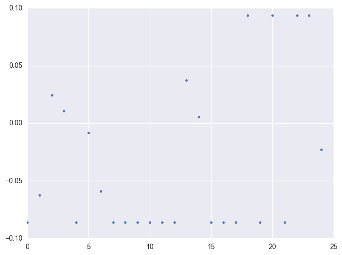
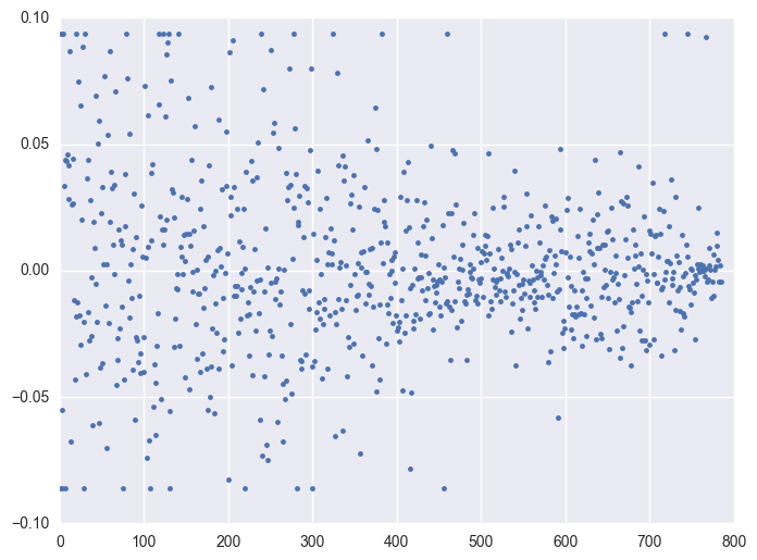
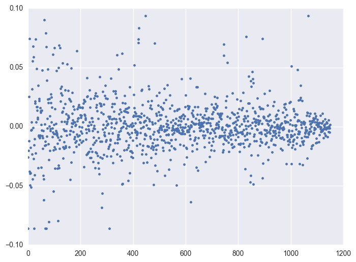
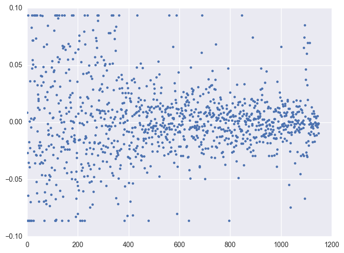
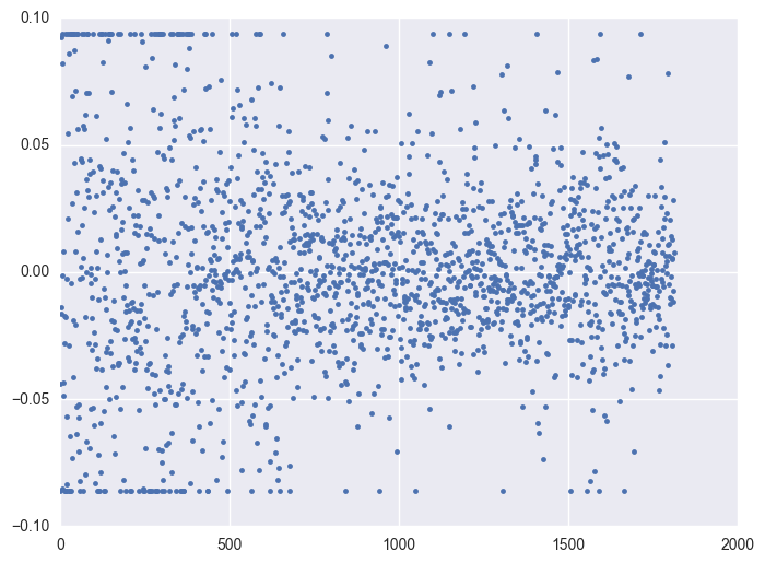
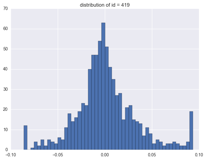
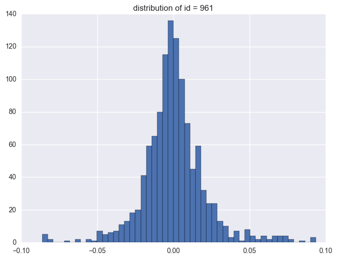
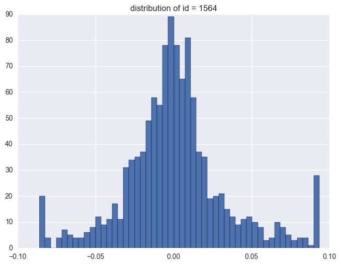
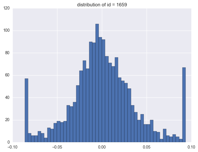
Take some instruments with outliers as example to plot y v.s. timestamp, there is the trend that at the starting time the data is more volatile, and it shows converging trend around 0. When the data converges to 0, the instrument will be stopped.
for i in df.query('(y >= 0.0934) | (y <= -0.0860)').id.unique()[:5]:
    plt.figure(figsize = (8, 6))
    df_sel = df.query('id == @i')
    plt.plot(df_sel.timestamp, df_sel.y, '.')
    plt.plot()
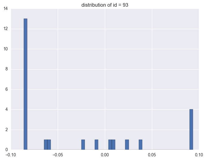
for i in df.query('(y >= 0.0934) | (y <= -0.0860)').id.unique()[:5]:
    print i
    df_sel = df.query('id == @i')
    plt.figure(figsize = (8, 6))
    plt.hist(df_sel.y, bins = 50)
    plt.title("distribution of id = {}".format(i))
    plt.plot()
93
419
961
1564
1659
1.3. timestamp
The next variable to study is timestamp. It indicates each transaction for each instrument. We will check the frequency of timestamp first. This will help us to understand at what time there are more transactions and when there are less transactions.
timestamp = df.timestamp
for bins in [100, 200]:
    plt.figure(figsize = (12, 9))
    plt.hist(timestamp, bins = bins)
    plt.xlabel("timestamp")
    plt.ylabel("data counts")
    plt.title("Histogram of timestamp: {} bins".format(bins))
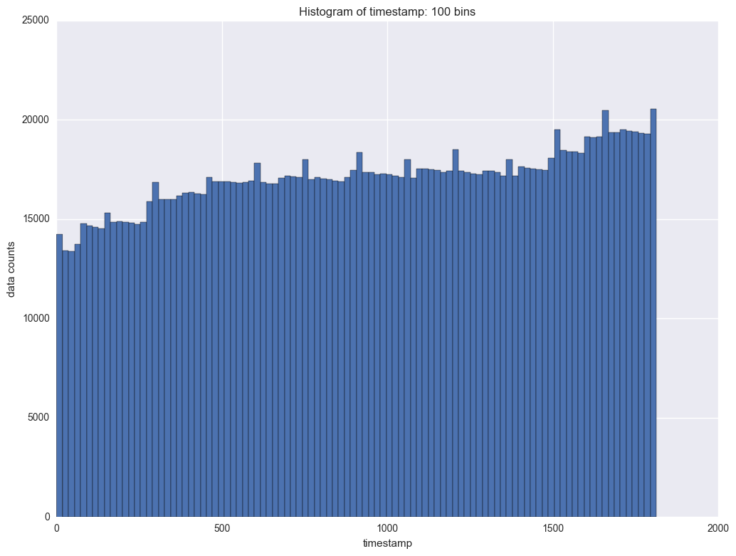
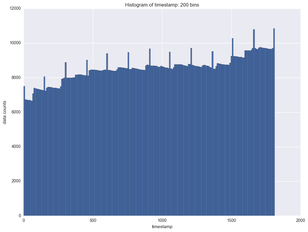
It shows there is period of the counts data by timestamp. In each period the counts will slightl decrease and then it will jump. The interval is about 100. So is it daily transaction and there are about 100 timestamps everyday?
1.4. Summary of data
-
There are 1424 unique id in the data, and there are 1813 unique timestamp in the data. within each id, the timestamp is unique.
-
some id only has a few transactions, while some id has more than 1000 transactions.
-
many independent variables has missing values. we need to impute missing values.
print len(df.id.unique())
print len(df.timestamp.unique())
1424
1813
2. More check of the data
2.1. is the timestamp unique for each instrument?
First I want to check for each id, if there are duplicated timestamp or not. The result shows there is no duplicated timestamp for each id. The way to do is group by each id, then compare the length of the subgroup and the counts of unique timestamp at each subgroup. we can define two functions and apply multiple self defined functons on the groupby object.
def f1(x):
    return [x.shape[0] , len(x.timestamp.unique())]

def f2(x):
    return {'shape': x.shape, 'uniq_cnt': len(x.timestamp.unique())}

print df.groupby('id').apply(f1).head()
print '\n'
print df.groupby('id').apply(f2).head()
id
0     [1646, 1646]
6       [728, 728]
7     [1543, 1543]
10      [116, 116]
11    [1813, 1813]
dtype: object


id
0     {u'shape': (1646, 111), u'uniq_cnt': 1646}
6       {u'shape': (728, 111), u'uniq_cnt': 728}
7     {u'shape': (1543, 111), u'uniq_cnt': 1543}
10      {u'shape': (116, 111), u'uniq_cnt': 116}
11    {u'shape': (1813, 111), u'uniq_cnt': 1813}
dtype: object
it shows in each id, the timestamp is unique. That is, there is only one obs for each id at each timestamp.
2.2. a little more about y and x
This is to show how to apply multiple funcitons on different columns. for y, we will calculate min, max and median within each instrument. for timestamp, check its counts; for a given x technical_40, calculate its non-null mean in each instrument to impute the missing values.
f0 = lambda x: x[~x.isnull()].mean()

f = {'y': ['min', 'max', 'median'], 'timestamp': ['size'], u'technical_40': {'fake name': f0}}

df.groupby('id').agg(f).head()
| y | timestamp | technical_40 | |||
|---|---|---|---|---|---|
| min | max | median | size | fake name | |
| id | |||||
| 0 | -0.086094 | 0.093498 | 0.000147 | 1646 | -0.071997 |
| 6 | -0.075099 | 0.057635 | -0.000100 | 728 | -0.091534 |
| 7 | -0.086094 | 0.093498 | -0.000009 | 1543 | -0.079504 |
| 10 | -0.086094 | 0.093498 | -0.002115 | 116 | -0.471554 |
| 11 | -0.086094 | 0.070152 | -0.000262 | 1813 | -0.115141 |
2.3. impute missing by median in each id group
As we shown above, lots of the x has missing values. A simple way to impute the missing value is its median. Here I will show how to impute all the missing values by the median value for each instrument, rather than using the median of the full data set.
fimpute = lambda x: x.fillna(x.median())

grp = df.groupby('id').apply(fimpute)

print grp.head()
           id  timestamp  derived_0  derived_1  derived_2  derived_3  \
id
0  131062   0        167  -0.064533   0.090540  -0.012166   0.009563
   131895   0        168  -0.064533   0.090540  -0.012166   0.009563
   132728   0        169  -0.064533   0.090540  -0.012166   0.009563
   133561   0        170  -0.230583   0.488096   0.935920   0.028222
   134393   0        171  -0.230583   0.488096   0.935920   0.028222

           derived_4  fundamental_0  fundamental_1  fundamental_2    ...     \
id                                                                   ...
0  131062   0.130775      -0.182136       0.502698       0.169803    ...
   131895   0.130775      -0.182136       0.502698       0.169803    ...
   132728   0.130775      -0.182136       0.502698       0.169803    ...
   133561  -0.083071      -0.240929       0.502698       0.212425    ...
   134393  -0.083071      -0.240929       0.502698       0.212425    ...

           technical_36  technical_37  technical_38  technical_39  \
id
0  131062      0.039496     -0.000043     -0.000002 -2.547840e-10
   131895      0.039496     -0.000043     -0.000002 -2.547840e-10
   132728      0.039496     -0.000043     -0.000002 -2.547840e-10
   133561      0.727659      0.000000      0.000000  0.000000e+00
   134393      0.727659      0.000000      0.000000  0.000000e+00

           technical_40  technical_41  technical_42  technical_43  \
id
0  131062     -0.071485     -0.000941  2.955212e-38     -0.000102
   131895     -0.071485     -0.000941  2.955212e-38     -0.000102
   132728     -0.071485     -0.000941  2.955212e-38     -0.000102
   133561     -0.160478     -0.000941  0.000000e+00      0.000000
   134393     -0.160478     -0.000941  0.000000e+00      0.000000

           technical_44         y
id
0  131062     -0.013518 -0.007108
   131895     -0.013518  0.001950
   132728     -0.013518  0.017724
   133561     -0.013518  0.012934
   134393     -0.013518 -0.025229

[5 rows x 111 columns]
df.columns[df.query('(id == 0) & (timestamp<170)').isnull().sum() == 0]
Index([u'id', u'timestamp', u'technical_22', u'technical_34', u'y'], dtype='object')
3. Correlation
3.1. check the correlation between x and y in the full data
numpy provide functition np.corrcoef() to calculate the pearson correlation coefficient and pandas has df.corr() to do the same thing. The better of pandas is it will handle missing values directly while numpy need to impute the missing first.
corr_d = {}
for i in df.columns:
    if i not in ['id', 'timestamp', 'y']:
        corr_d[i] = df.ix[:, [i, 'y']].corr().ix[0, 1]
corr = pd.DataFrame.from_dict(corr_d, orient = "index").sort_values(0)

print corr.head()
print corr.tail()
                     0
technical_20 -0.016534
technical_27 -0.008092
technical_19 -0.007647
technical_35 -0.006009
technical_36 -0.005902
                       0
fundamental_18  0.005123
fundamental_53  0.006009
fundamental_51  0.006013
fundamental_11  0.008151
technical_30    0.014272
as is shown, the correlation between all x and y are not low. The most negative correlated variables are technical_20(-0.016534), tenichical_27(-0.008092); the most positive correlated variables are fundamental_18 (0.005123), fundamental_53(0.006009). The maximum correlation is less them 2%.
Let's have a look at within each time stamp, if there is any variables have strong correlation with y.
3.2. correlation between x and y within timestamp
The direct correlation between x and y is very low. However, since the data is the combination of each instrument, the intuitive think is to check the correlation of y and x within each instrument. Data can also be treated as multiple instrments at each time stamp, so another thought is to check the correlation within each timestamp.
grp = df.groupby('timestamp')
s1 = []
s2 = []
for i, (k, g) in enumerate(grp):
    for c in g.columns:
        if c not in ['id', 'timestamp', 'y']:
            s1.append((k, c))
            s2.append(g.ix[:, [c, 'y']].corr().ix[0, 1])
After we sort the value, we can see that for for timestamp 679 and 359, technical_40 has the highest correlation with y; for timestamp 679, technical_7 has the highest correlation.
ssort = sorted([list(i) + [j] for i, j in zip(s1, s2)], key = lambda x: x[2])
print ssort[:5]
print '\n'
print ssort[-5:-1]
[[679, u'technical_40', -0.61238033073603038], [359, u'technical_40', -0.60861802020416578], [679, u'technical_7', -0.6031429961412077], [1500, u'technical_36', -0.50500188603013252], [513, u'technical_20', -0.50077160906865514]]


[[239, u'fundamental_59', 0.58286085236367469], [239, u'technical_22', 0.62048394512745275], [241, u'technical_40', 0.64763093025619489], [239, u'technical_7', 0.69531703280170543]]
For timestamp=679, techinicatl_40 has strong negative correlation(-0.61238033073603038) with y. For stimestamp=359, it is also techinical_40 has strong negative corrleation(-0.60861802). So although overll the correlation is weak, but if we look at the data with in each timestamp group, we can find some variables that has pretty storng correlation with y.
3.3. correlation between x and y within id
For each instrument, we can check which variables have the highest correlation with y. This will be the correlation within each group by instrument id.
grp = df.groupby('id')
s1 = []
s2 = []
for i, (k, g) in enumerate(grp):
    for c in g.columns:
        if c not in ['id', 'timestamp', 'y']:
            s1.append((k, c))
            s2.append(g.ix[:, [c, 'y']].corr().ix[0, 1])
It shows the correlation between x and y within each instrument is also higher then the correlation of the full data, although it is not as strong as group by timestamp.
ssort = sorted([list(i) + [j] for i, j in zip(s1, s2)], key = lambda x: x[2], reverse=True)
print ssort[:5]
print '\n'
print ssort[-5:-1]
[[10, u'technical_5', 0.30671451385776877], [10, u'technical_2', 0.20053930725042707], [10, u'fundamental_61', 0.19872930349160989], [10, u'fundamental_57', 0.16555170011275736], [10, u'fundamental_63', 0.15923680951545652]]


[[2158, u'technical_35', -0.30463890005790334], [2158, u'technical_31', -0.40696077297260669], [2158, u'technical_42', nan], [2158, u'technical_43', nan]]
For instrument 10, technical_5 has positive correlation(0.306714513) with y. instrument 2158, techinical_35 has negative correlation with y.
So we we study each instrument independently, we still get stronger correlation than using the whole data. This information will be helpful later in building the model.
from operator import itemgetter, attrgetter, methodcaller
sorted([list(i) + [j] for i, j in zip(s1, s2)], key=itemgetter(0, 2))
# sorted([list(i) + [j] for i, j in zip(s1, s2)], key=attrgetter('correlation'))
3.4. Summary
If we take the full data, the correlation between all the x and y is very weak. However, if we group the data by instrument or by the timestamp, the correlation will be stronger.
But can we group the data for modeling?
4. Model
4.1. models on full data
Since y is (capped and floored) continuous variable, the easiest model is to build the linear regression model.3 regression will be compared: linear regression, ridge regression and lasso regression. The difference between redige and lasso is in the penalty function. Ridge is two order penalty function while lasso is absolute penalty function. Thus lasso can select variables by letting these coefficients appreach 0 but ridge regression cannot.Adaboost regressor is also tested. When building classification models, adaboost is thought to be the best out of pocket model. Here in the regression models, its performance is not that better comparing to linear gression.
Full data has beed used without variable selection. It shows linear regression has the best mean squared errors.
from sklearn.cross_validation import train_test_split
from sklearn import linear_model
from sklearn.tree import DecisionTreeRegressor
from sklearn.ensemble import AdaBoostRegressor
from sklearn.metrics import mean_squared_error

lr = linear_model.LinearRegression()
ridge = linear_model.Ridge()
lasso = linear_model.Lasso()
df.timestamp.unique()
dfx_median = df.ix[:, 2:100].median()
import time
st = time.time()
lr.fit(df.ix[:, 2:100].fillna(dfx_median), df['y'])
print mean_squared_error(lr.predict(df.ix[:, 2:100].fillna(0)), df['y'])

ridge.fit(df.ix[:, 2:100].fillna(dfx_median), df['y'])
print mean_squared_error(ridge.predict(df.ix[:, 2:100].fillna(0)), df['y'])

lasso.fit(df.ix[:, 2:100].fillna(dfx_median), df['y'])
print mean_squared_error(lasso.predict(df.ix[:, 2:100].fillna(0)), df['y'])


reg_ada = AdaBoostRegressor(DecisionTreeRegressor(max_depth = 4), n_estimators = 20)
reg_ada.fit(df.ix[:, 2:100].fillna(dfx_median), df['y'])
print mean_squared_error(reg_ada.predict(df.ix[:, 2:100].fillna(0)), df['y'])

ed = time.time()

print ed-st
Of course this comparison is too raw to use since we put all data as training data and compare result from the training data. Usually if you try to overfit the model, the performance on the training data will be good but the prediction power of the model will not as good as expected. We should build a model to predict the trend rather than to predict the errors from the training data.
To compare the model performance more reasonable, we should split the data to training data and validation data. Building model on the training data and comparing model on the validation data.
In the above example all variables are used in the model. In fact this is not a good way either. One consern is incaluding too many variables will cause overfitting.Generally the more variables included, better performance will the training model performance be. The second is when there are a lot of variables, some variables may be high correlated, resulting in multi-collinearity. The third thing is including too many variables will cost lots of resources to fit the model.
4.2. Split to training/validation and pick 20 most related vars
From the correlation between x and y we can pick the top 20 variables by the correlation with y. The full data will be split to 60% as training data and 40% as validaiton data. As we can see, the running time is much shorter than using the all the x. Linear regression is the best model. For most cases, the MSE will be lower than using all the variables in the model.
top20 = corr[0].map(lambda x: abs(x)).sort_values(ascending = False)[:20].index

dfx_median = df.median()
df2 = df.fillna(dfx_median)

x_train, x_test, y_train, y_test = train_test_split(df2.ix[:, top20], df2['y'], test_size=0.4, random_state=0)


lr = linear_model.LinearRegression()
ridge = linear_model.Ridge()
lasso = linear_model.Lasso()

st = time.time()

lr.fit(x_train, y_train)
print mean_squared_error(lr.predict(x_test), y_test)

ridge.fit(x_train, y_train)
print mean_squared_error(ridge.predict(x_test), y_test)

lasso.fit(x_train, y_train)
print mean_squared_error(lasso.predict(x_test), y_test)

reg_ada = AdaBoostRegressor(DecisionTreeRegressor(max_depth = 4), n_estimators = 20)
reg_ada.fit(x_train, y_train)
print mean_squared_error(reg_ada.predict(x_test), y_test)

ed = time.time()

print ed-st
0.000500598917586
0.000500607067788
0.000500847186479
0.00050218493994
90.745000124
4.3. model on each group
Using the top 20 correlated coclumns will improve the model a little. The correlation is stronger amont the group: by instrument or by timestamp. So if building a model for each timestamp, will it improve more?
Let's look at the example of building the model on each timestamp and select the top 10 correlated variables.
pred_lr = []
pred_ridge = []
pred_lasso = []

for i in df.timestamp.unique():
    if i % 300 == 0:
        print i
    df0 = df.query('timestamp == @i')
    df0 = df0.fillna(df0.median())
    select_var =  df0.ix[:, 2:-1].corrwith(df0.y).dropna().map(lambda x: abs(x)).sort_values()[-10:].index
    #print select_var

    lr.fit(df0.ix[:, select_var], df0['y'])
    ridge.fit(df0.ix[:, select_var], df0['y'])
    lasso.fit(df0.ix[:, select_var], df0['y'])

    pred_lr = np.r_[pred_lr, lr.predict(df0.ix[:, select_var])]
    pred_ridge = np.r_[pred_ridge, ridge.predict(df0.ix[:, select_var])]
    pred_lasso = np.r_[pred_lasso, lasso.predict(df0.ix[:, select_var])]
0
300
600
900
1200
1500
1800
print mean_squared_error(pred_lr, df['y'])
print mean_squared_error(pred_ridge, df['y'])
print mean_squared_error(pred_lasso, df['y'])
0.000414826716159
0.000419801804688
0.00048255088499
Above are some exploratory analysis of the data and the tentative models. The more detailed models should be built on the consideration above and the variable selection.