上一篇文章，我们使用tensorflow(TF)来建立了一个单feature的线性回归模型。给定feature的值（house size），我们可以预测出房屋价格。

我们回顾一下上一章怎么做的：

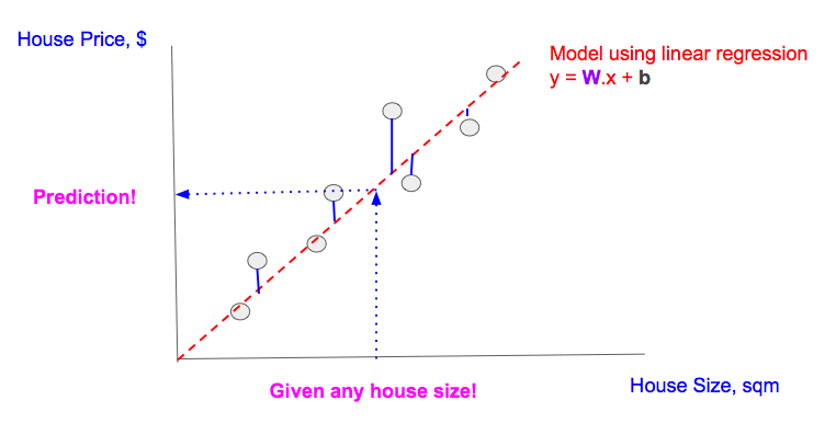
1. 我们有房屋面积和房屋价格的数据（图中灰色原点）

2. 用线性回归来建模（红色虚线）

3. 通过最小化损失函数（图中蓝线的长度的平方和）来找出最优的模型的W和b

4. 给定房屋面积，应用建立的线性模型来预测房屋价格（图中蓝色虚线对应的点）

在机器学习的论文中，我们经常会遇到‘training’这个词。我们首先来看看在TF中它的含义。

线性回归模型

Linear Model (in TF notation): y = tf.matmul(x,W) + b

线性回归的目的是找出W和b,对给定的feature值(x),当我们把W,b和x带入模型，我们可以得到prediction(y)。

要得到W和b，我们需要用给定的数据(真实的feature值x和真实的结果y_， 注意y_的下划线)来训练(train)模型。

Training Illustrated

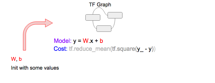
要找到最优的W和b，我们需要定义一个损失函数用来衡量对某一个给定的feature（x）值，预测值（y）和真实值(y_)之间的差异。为了简化，我们用最小平方差的和(MSE)作为损失函数。

Cost function (in TF notation): tf.reduce_mean(tf.square(y_ - y))

通过最小化损失函数，我们可以得到好的W和b的值。

用来做训练的程序代码非常简单，我们用[A,B,C,D]来标记各个部分。下面将会用到。

# ... (snip) Variable/Constants declarations (snip) ...
# [A] TF.Graph
y = tf.matmul(x,W) + b
cost = tf.reduce_mean(tf.square(y_-y))
# [B] Train with fixed 'learn_rate'
learn_rate = 0.1
train_step =
    tf.train.GradientDescentOptimizer(learn_rate).minimize(cost)
for i in range(steps):
  # [C] Prepare datapoints
  # ... (snip) Code to prepare datapoint as xs, and ys (snip) ...
  # [D] Feed Data at each step/epoch into 'train_step'
  feed = { x: xs, y_: ys }
  sess.run(train_step, feed_dict=feed)

A当中的线性模型和损失函数可以被表示成下面的TF流程图

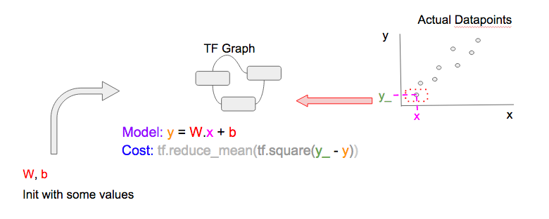
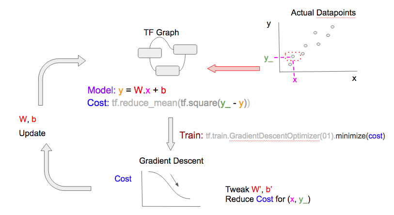
下一步，我们要选择一个C当中的数据(x, y_)，输入到D当中来得到预测值(y)和损失函数。TF流程图如下：

要得到更好的W和b，我们在B中通过tf.train.GradientDescentOptimizer做梯度下降来得到损失函数。更简易的说法是：给定当前的损失值，根据图中别的变量（W和b）所得到的损失函数的值，优化器会对W和b做一个小变化（增加/减少），从而使得对那一个数据点的预测值更好。

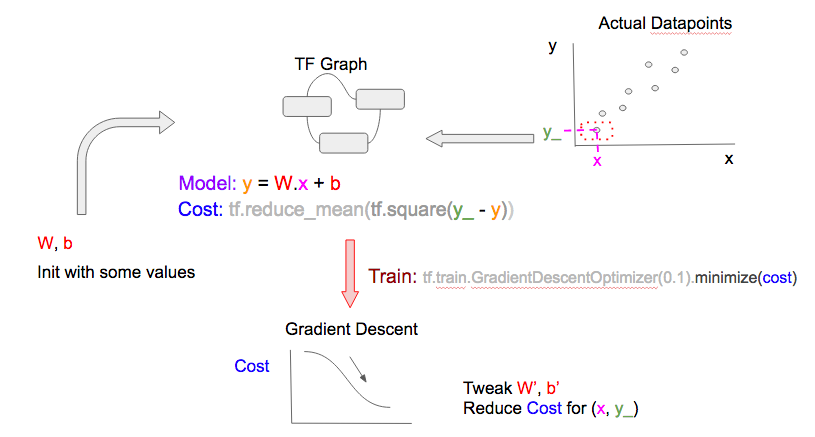
最后一步就是更新调整过的W和b的值。注意这一个周期(cycle)在机器学习的文档中也叫epoch。

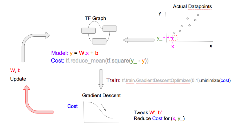
在下一个epoch，重复以上步骤，但是用一个不同的数据点(x, y_)

使用不同的数据点来建模，所得到的W和b就可以用来预测任意的feature。注意

• 大部分时候，更多的数据点得到的模型会更好

• 如果你的epochs比你的数据点还多，你可以重复利用数据点，这是没有问题的。梯度下降的优化器总是使用数据点和损失函数(从相应的epoch中的W和b和数据点计算出来)来调整W和b。优化器可能已经用过这个数据点，但是因为损失函数不同，所以它仍然会得到新的信息，也会得到新的调整过的W和b。

你可以训练你的模型给定次数的epoch，或者直到损失函数低于某个给定的值。

Training variation

stochastic，mini-batch, batch

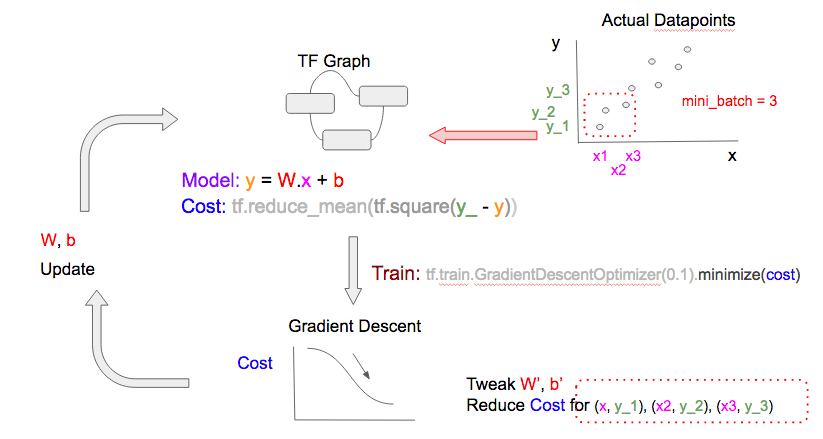
在上面的模型训练中，我们每次输入一个数据点。这叫做随机梯度下降(stochastic gradient descent)。我们也可以在每个epoch中输入一批数据点，这叫做mini-batch gradient descent。甚至我们可以在每个epoch中输入所有的数据点，这叫做batch gradient descent。请看下面的比较图示。注意这三个图有两个不同

• 每个epoch中输入到TF.Graph的数据点(右上角的数据点)不同
• 用来调整W和b的梯度下降优化器所用到的数据点（右下角）也不相同

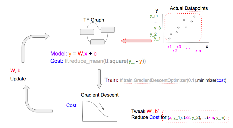
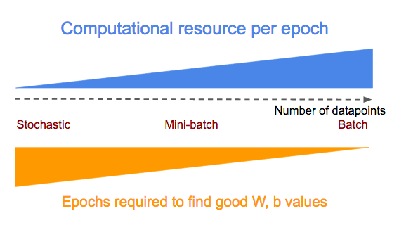
在每个epoch中使用到的数据点有两层含义。如果每个epoch使用更多的数据点：

• 计算损失函数和梯度下降的计算资源(加减乘)会减少
• 模型学习的速度会提高

使用stochastic, mini-batch, batch gradient descent 的优缺点见下图

要在stochastic, mini-batch, batch gradient descent这三个办法中切换，我们只需要在下面的[C]当中设置不同的batch大小，然后根据batch大小把对应的batch的数据点输入到模型训练[D]中。

# * all_xs: All the feature values
# * all_ys: All the outcome values
# datapoint_size: Number of points/entries in all_xs/all_ys
# batch_size: Configure this to:
#             1: stochastic mode
#             integer < datapoint_size: mini-batch mode
#             datapoint_size: batch mode
# i: Current epoch number
if datapoint_size == batch_size:
  # Batch mode so select all points starting from index 0
  batch_start_idx = 0
elif datapoint_size < batch_size:
  # Not possible
  raise ValueError(“datapoint_size: %d, must be greater than         
                    batch_size: %d” % (datapoint_size, batch_size))
else:
  # stochastic/mini-batch mode: Select datapoints in batches
  #                             from all possible datapoints
  batch_start_idx = (i * batch_size) % (datapoint_size — batch_size)
  batch_end_idx = batch_start_idx + batch_size
  batch_xs = all_xs[batch_start_idx:batch_end_idx]
  batch_ys = all_ys[batch_start_idx:batch_end_idx]


# Get batched datapoints into xs, ys, which is fed into
# 'train_step'
xs = np.array(batch_xs)
ys = np.array(batch_ys)

Learn Rate的变化

学习速度(Learn Rate)指的是梯度下降来调整W和b的这时候，每次增加或者减小的大小。当learn rate比较小的时候，前进速度会很慢，但是会渐渐收敛到最小损失函数值。当learn rate比较大的时候，达到最小损失函数的速度会比较快，但是有可能会走过头，导致找不到最小值。

要克服这一点，肯多ML的实际操作是开始的时候用比较大的learn rate（假设初始的损失函数离最小值比较远），然后每个epoch渐渐减小learn rate以防止走过头。

TF提供了两个办法。这个StackOverflow thread讲的非常棒。总结如下:

使用变化的learn rate的梯度下降优化器

TF提供了不同的支持learn rate变化的梯度下降优化器，比如tf.train.AdagradientOptimizer和tf.train.AdamOptimizer.

使用tf.placeholder建Learn Rate

如前所述，我们在tf.train.GradientDescentOptimizer当中用tf.placeholder来申明Learn Rate的时候，我们可以在每个epoch中输入不同的值。这类似于在每个epoch中我们用tf.placeholders来输入不同的数据点到x, y_。

这样做需要两个小的改动:

# Modify [B] to make 'learn_rate' a 'tf.placeholder'
# and supply it to the 'learning_rate' parameter name of
# tf.train.GradientDescentOptimizer
learn_rate = tf.placeholder(tf.float32, shape=[])
train_step = tf.train.GradientDescentOptimizer(
    learning_rate=learn_rate).minimize(cost)
# Modify [D] to include feed a 'learn_rate' value,
# which is the 'initial_learn_rate' divided by
# 'i' (current epoch number)
# NOTE: Oversimplified. For example only.
feed = { x: xs, y_: ys, learn_rate: initial_learn_rate/i }
sess.run(train_step, feed_dict=feed)

总结

我们演示了机器学习的训练是什么意思，以及在Tensorflow中怎么定义模型和损失函数。然后通过输入数据点到梯度下降优化器，进行循环来得到W和b的值。我们还讨论了训练过程中两个常见的变化：每个epoch中使用不同的数据集的大小，以及使用不同的learn rate。

下一章

• 设置Tensor Board来可视化TF的执行，这样可以检测到我们模型，损失函数和梯度下降的问题
• 展示一个多特征(features)的线性回归模型

Reference

1. Gentlest Introduction to Tensorflow #2