%matplotlib inline
import math,sys,os,numpy as np, pandas as pd
from numpy.linalg import norm
from PIL import Image
from matplotlib import pyplot as plt, rcParams, rc
from scipy.ndimage import imread
from skimage.measure import block_reduce
import cPickle as pickle
from scipy.ndimage.filters import correlate, convolve
from ipywidgets import interact, interactive, fixed
from ipywidgets.widgets import *
rc('animation', html='html5')
rcParams['figure.figsize'] = 3, 6
%precision 4
np.set_printoptions(precision=4, linewidth=100)
1. convolve and correlate in numpy
1.1. convolve of two vectors
The convolution of two vectors, u and v, represents the area of overlap under the points as v slides across u. Algebraically, convolution is the same operation as multiplying polynomials whose coefficients are the elements of u and v.
Let m = length(u) and n = length(v) . Then w is the vector of length m+n-1 whose kth element is \(w(k)=\sum_j u(j)v(k−j+1)\).
The sum is over all the values of j that lead to legal subscripts for u(j) and v(k-j+1), specifically j = max(1,k+1-n):1:min(k,m). When m = n, this gives
w(1) = u(1)*v(1)
w(2) = u(1)*v(2)+u(2)*v(1)
w(3) = u(1)*v(3)+u(2)*v(2)+u(3)*v(1)
...
w(n) = u(1)*v(n)+u(2)*v(n-1)+ ... +u(n)*v(1)
...
w(2*n-1) = u(n)*v(n)
np.convolve([1,2], [3,4,5])
array([ 3, 10, 13, 10])
3 = 1 * 3
10 = 1 * 4 + 2 * 3
13 = 1 * 5 + 2 * 4
10 = 2 * 5
convolve([1,2], [3,4,5])
array([15, 19])
1.2. correlate of two vectors
c_{av}[k] = sum_n a[n+k] * conj(v[n])

The definition of correlation above is not unique and sometimes correlation may be defined differently. Another common definition is:

c'_{av}[k] = sum_n a[n] conj(v[n+k])
which is related to c_{av}[k] by c'_{av}[k] = c_{av}[-k].
numpy.correlate(a, v, mode='valid', old_behavior=False)[source]
Cross-correlation of two 1-dimensional sequences.
This function computes the correlation as generally defined in signal processing texts:
z[k] = sum_n a[n] * conj(v[n+k])
with a and v sequences being zero-padded where necessary and conj being the conjugate.
np.correlate([1,2,3], [4,5,6], mode = 'full')
array([ 6, 17, 32, 23, 12])
 0 lag: 32 = 1 * 4 + 2 * 5 + 3 * 6
 1 lag: 23 = 2 * 4 + 3 * 5
 2 lag: 12 = 3 * 4
-1 lag: 17 = 1 * 5 + 2 * 6
-2 lag: 6 = 1 * 6
correlate([1,2,3], [4,5,6])
array([21, 32, 41])
np.correlate([1,2], [3,4,5], mode = 'full')
array([ 5, 14, 11, 6])
 0 lag: not same length, not available
 1 lag: 11 = 1 *3 + 2 * 4
 2 lag:  6 = 2 * 3
-1 lag: 14 = 1 * 4 + 2 * 5
-2 lag:  5 = 1 * 5
2. read and plot image in matplotlib
2.1. Color image
An image from a standard digital camera will have a red, green and blue channel(RGB). A grayscale image has just one channel.
So if a color image is read in, the data will have three dimensions: width, height and chanels. And number of chanels(the 3rd dimension) all the time is three. For a grayscale image, the number of chanels will be one.
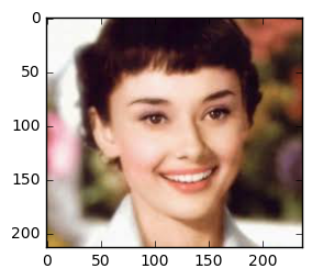
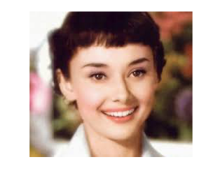
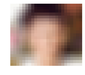
For example, the following Cherry blossom will have dimension of (, , ) and the third dimension is 3.
# read in an image and show the image inline
im = plt.imread("heben.jpg")#r"Vd-Orig.png")
print im.shape
plt.imshow(im)
(213L, 237L, 3L)


<matplotlib.image.AxesImage at 0x13775860>
im[:10, :10, 1]
array([[247, 247, 247, 247, 247, 247, 247, 247, 249, 249],
       [247, 247, 247, 247, 247, 247, 247, 247, 249, 249],
       [248, 248, 248, 248, 248, 248, 248, 248, 249, 249],
       [248, 248, 248, 248, 248, 248, 248, 248, 249, 249],
       [249, 249, 249, 249, 249, 249, 249, 249, 249, 249],
       [249, 249, 249, 249, 249, 249, 249, 249, 249, 249],
       [249, 249, 249, 249, 249, 249, 249, 249, 249, 249],
       [250, 250, 250, 250, 250, 250, 250, 250, 249, 249],
       [248, 248, 248, 248, 248, 248, 248, 248, 248, 248],
       [248, 248, 248, 248, 248, 248, 248, 248, 248, 248]], dtype=uint8)
We can also only show one chanel of the image. For example, the following is only the 3rd chanel of the image.
# only show the third chanel (index 2)
plt.imshow(im[:, :, [0,0,0]].astype(dtype="uint8"))
<matplotlib.image.AxesImage at 0x1971e898>
plt.imshow(im[:, :, 2].astype(dtype="uint8"))
<matplotlib.image.AxesImage at 0x163bca58>
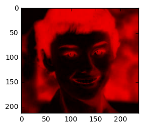
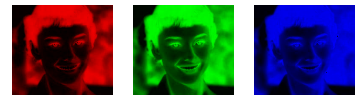
Another useful method is to plot the red(or green, blue) chanel only in the graph. To do that, we will keep only that chanel data, and set the rest of the chanel as 0.
tmp_im = np.zeros(im.shape)
tmp_im[:, :, 0] = im[:, :, 0]
plt.imshow(tmp_im)
tmp_im[:3, :3, :]
array([[[ 247.,    0.,    0.],
        [ 247.,    0.,    0.],
        [ 247.,    0.,    0.]],

       [[ 247.,    0.,    0.],
        [ 247.,    0.,    0.],
        [ 247.,    0.,    0.]],

       [[ 248.,    0.,    0.],
        [ 248.,    0.,    0.],
        [ 248.,    0.,    0.]]])
def plti(im, **kwargs):
    plt.imshow(im, interpolation="none", **kwargs)
    plt.axis('off') # turn off axis
    plt.show()

im = im[:, :, :]  # slice
plti(im)
fig, axs = plt.subplots(nrows=1, ncols=3, figsize=(15,5))

for c, ax in zi//figures/[png](/figures/range(3), axs):
    tmp_im = np.zeros(im.shape)
    tmp_im[:,:,c] = im[:,:,c]
    one_channel = im[:,:,c].flatte//figures/[png](/figures/)
    print("channel", c, " max = ", max(one_channel), "min = ", mi//figures/[png](/figures/one_channel))
    ax.imshow(tmp_im)
    ax.set_axis_off()
plt.show()
('channel', 0, ' max = ', 255, 'min = ', 15)
('channel', 1, ' max = ', 255, 'min = ', 1)
('channel', 2, ' max = ', 255, 'min = ', 0)
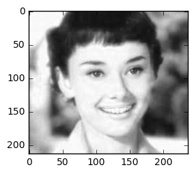
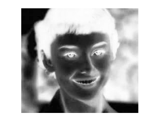
2.2. Grayscale image
To convert a color image to grayscale, the 3 chanels data of RGB will be weighted sumed to one dimension. The weights is the average of the 3 chanels data by np.mea//figures/[png](/figures/im, axis = (0, 1)).
im_mean = np.mea//figures/[png](/figures/im, axis = (0, 1))
print im_mean / sum(im_mean)

def to_grayscale(im, weights = np.c_[0.3445, 0.3081, 0.3474]):
    """
    Transforms a colour image to a greyscale image by
    taking the mean of the RGB values, weighted
    by the matrix weights
    """
    tile = np.tile(weights, reps=(im.shape[0], im.shape[1], 1))
    return np.sum(tile * im, axis=2)

img = to_grayscale(im, np.c_[0.3957, 0.325, 0.2793])

plti(img, cmap='Greys')
[ 0.4002 0.3167 0.2831]
3. Convolve over image
In image processing, convolution matrix is a matrix that each element will be multiplied by the part of the matrix that is been convolved.
For example, matrix A is of dimension 10*10, matrix B which is the conversion matrix of dimension 3 * 3. The convolution of B over A means for each 3 * 3 subset in A(or maybe zero padding of A), do the elementwise multiply between the subset and B, then the sum of the multiply will be the corresponding element in the output matrix. More details will be introduced later.
There will be some corresponding question when we do the above calculation: 1. how to pick the dimension of B? 2. How many stride shall we skip when selecting the subset? 3. what kind of zero-padding shall be used? These questions will be answered later.
The following is an example of convolution matrix called window with shape 5 * 5, with all elements equal and the sum is 1.Since its weights are all the same, this will mask the image.
### convolve to mask the image

from scipy.signal import convolve2d
from scipy.ndimage.interpolation import zoom

im_small = zoom(im, (0.1, 0.1, 1))

def convolve_all_colours(im, window):
    """
    Convolves im with window, over all three colour channels
    """
    ims = []
    for d in range(3):
        im_conv_d = convolve2d(im[:,:,d], window, mode="same", boundary="symm")
        ims.append(im_conv_d)

    im_conv = np.stack(ims, axis=2).astype("uint8")

    return im_conv

n = 5
window = np.ones((n,n))
window /= np.sum(window)
plti(convolve_all_colours(im_small, window))
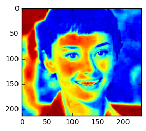
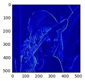
Some more interesting convolution matrix: edge detection
from numpy import *
import scipy
from scipy import misc, ndimage

def detect_edges(image,masks):
    edges=zeros(image.shape)
    for mask in masks:
        edges=maximum(scipy.ndimage.convolve(image, mask), edges)
    return edges

image=plt.imread("lenna.png")

Faler=[ [[-1,0,1],[-1,0,1],[-1,0,1]],
        [[1,1,1],[0,0,0],[-1,-1,-1]],
    [[-1,-1,-1],[-1,8,-1],[-1,-1,-1]],
    [[0,1,0],[-1,0,1],[0,-1,0]] ]

edges=detect_edges(image, Faler)
plt.imshow(edges)
<matplotlib.image.AxesImage at 0x1be16f28>
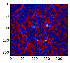
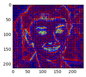
plt.imshow(correlate(im[:, :, 0], [[1, 0, -1], [0,0,0], [-1,0,1]]))
<matplotlib.image.AxesImage at 0x1b7a9908>
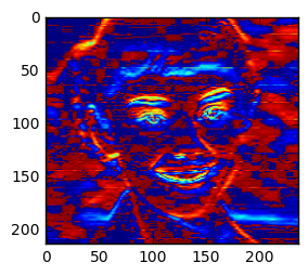
plt.imshow(correlate(im[:, :, 0], [[-1, -1, -1], [1,1,1], [0,0,0]]))
<matplotlib.image.AxesImage at 0x132a69e8>
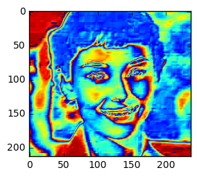
plt.imshow(correlate(im[:, :, 0], [[-1, -1, -1], [-1,8,-1], [-1,-1,-1]]))
<matplotlib.image.AxesImage at 0x1233a320>
im1 = correlate(im[:, :, 2], [[1, 1, 0], [1,0,1], [0, -1, -1]])
im2 = convolve(im[:, :, 2], np.rot90([[1, 1, 0], [1,0,1], [0, -1, -1]],2))

print np.allclose(im1, im2)

plt.imshow(im1)
True


<matplotlib.image.AxesImage at 0xf6fa860>

plt.imshow(im2)
<matplotlib.image.AxesImage at 0x10505470>
Reference
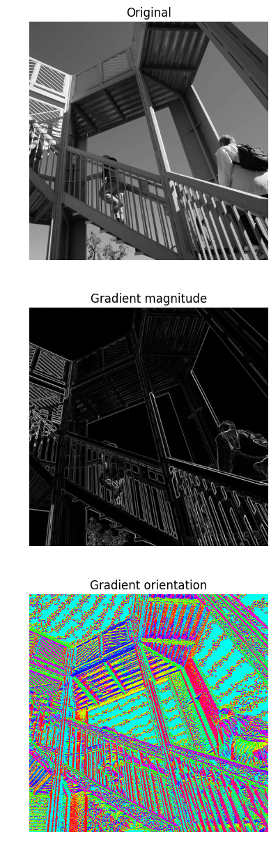
from scipy import signal
from scipy import misc
print ascent.shape
scharr = np.array([[ -3-3j, 0-10j,  +3 -3j],
                   [-10+0j, 0+ 0j, +10 +0j],
                   [ -3+3j, 0+10j,  +3 +3j]]) # Gx + j*Gy
grad = signal.convolve2d(ascent, scharr, boundary='symm', mode='same')


import matplotlib.pyplot as plt
fig, (ax_orig, ax_mag, ax_ang) = plt.subplots(3, 1, figsize=(6, 15))
ax_orig.imshow(ascent, cmap='gray')
ax_orig.set_title('Original')
ax_orig.set_axis_off()
ax_mag.imshow(np.absolute(grad), cmap='gray')
ax_mag.set_title('Gradient magnitude')
ax_mag.set_axis_off()
ax_ang.imshow(np.angle(grad), cmap='hsv') # hsv is cyclic, like angles
ax_ang.set_title('Gradient orientation')
ax_ang.set_axis_off()
fig.show()
(512L, 512L)