0. Description
This data contains the recordings of a series of borrowers(based on id) from 2015-01-01 to 2015-11-02. The target variable is a categorical variable with value 0 or 1. target=1 means the borrower is default, otherwise it means the borrower is active. Totally there are 1168 unique borrower id.
Each borrower will have one recording or no recording everyday. The minimum number of recording is 3 and the maximum number of recording is 304.
For each recording, there are 9 independent variables named as x1 to x9.
The job is to predict the target variable based on the independent variables.
1. Data View
The data looks like
| date | id | target | x1 | x2 | x3 | x4 | x5 | x6 | x7 | x8 | x9 | |
|---|---|---|---|---|---|---|---|---|---|---|---|---|
| 0 | 2015-01-01 | S1F01085 | 0 | 215630672 | 56 | 0 | 52 | 6 | 407438 | 0 | 0 | 7 |
| 1 | 2015-01-01 | S1F0166B | 0 | 61370680 | 0 | 3 | 0 | 6 | 403174 | 0 | 0 | 0 |
| 2 | 2015-01-01 | S1F01E6Y | 0 | 173295968 | 0 | 0 | 0 | 12 | 237394 | 0 | 0 | 0 |
| 3 | 2015-01-01 | S1F01JE0 | 0 | 79694024 | 0 | 0 | 0 | 6 | 410186 | 0 | 0 | 0 |
| 4 | 2015-01-01 | S1F01R2B | 0 | 135970480 | 0 | 0 | 0 | 15 | 313173 | 0 | 0 | 3 |
| 5 | 2015-11-02 | Z1F0MA1S | 0 | 18310224 | 0 | 0 | 0 | 10 | 353705 | 8 | 8 | 0 |
| 6 | 2015-11-02 | Z1F0Q8RT | 0 | 172556680 | 96 | 107 | 4 | 11 | 332792 | 0 | 0 | 13 |
| 7 | 2015-11-02 | Z1F0QK05 | 0 | 19029120 | 4832 | 0 | 0 | 11 | 350410 | 0 | 0 | 0 |
| 8 | 2015-11-02 | Z1F0QL3N | 0 | 226953408 | 0 | 0 | 0 | 12 | 358980 | 0 | 0 | 0 |
| 9 | 2015-11-02 | Z1F0QLC1 | 0 | 17572840 | 0 | 0 | 0 | 10 | 351431 | 0 | 0 | 0 |
- Target Variable: target is the categorical variable with values 0 and 1
- Independent Variables: we can use all the other variables as the independent variables, including x1 to x9, even date and id if with proper transformation.
Some Observations:
-
From the data we can see
x1andx6are like numeric variable while the others are like categorical variable. We will do some analysis later. -
x2,x3,x7,x8,x9has lots of zeros -
The first 3 characters of id might be useful to distinguish the target variable
-
The variable date might be useful: we can get month information which might be useful, or we can get the time duration from first recording time to positive target time
Some Extras:
- Totally there are 124494 rows in the data. But there are only 1168 unique ids.
- Overall there are only 106 target=1. That is, the rate is about 0.08%.
- Each id only has at most one time target=1.
1.1. Data summary and target info
There are 124494 rows of data in all but there is only 106 target=1. So the data is very inbalanced.
import pandas as pd
import matplotlib.pyplot as plt
import seaborn as sns
import numpy as np
import seaborn as sns

from sklearn.ensemble import RandomForestClassifier, AdaBoostClassifier, GradientBoostingClassifier, ExtraTreesClassifier
from sklearn.svm import SVC, LinearSVC
from sklearn.metrics import confusion_matrix
from sklearn.cross_validation import KFold
from sklearn.model_selection import train_test_split, StratifiedShuffleSplit
from sklearn.metrics import log_loss

import plotly.offline as py
py.init_notebook_mode(connected=True)
import plotly.graph_objs as go
import plotly.tools as tls

%matplotlib inline
#get_ipython().magic('matplotlib inline')
plt.rcParams['figure.figsize'] = (20, 16)

mypath = r'/home/shm/projects/blog_study_draft/data//'
indata = pd.read_csv(mypath + r'defaults.csv')
print(indata.shape)
print(indata.target.sum())
(124494, 12)
106
1.2. Borrowers defaulted
Since there are many target=0. We will check how many borrowers defaulted and how many not.
It shows there are 106 borrowers defaulted. The rest 1062 borrowers did not have any default during this observation time period.
defaultid = indata[indata.target == 1].id.unique()

print(indata[indata.id.isin(defaultid)].id.unique().shape)
print(indata[~indata.id.isin(defaultid)].id.unique().shape)
print(indata.id.unique().shape)
(106,)
(1062,)
(1168,)
For furture use, I will pick out the defaulted borrowers to a standalone data set.
defaults = indata[indata.id.isin(defaultid)]
print(defaults.shape)
(10713, 12)
2. Data Engineering
2.1. Unique values for each variable
The data does not have a dictionary to indicate clearly what does the x mean. I will determine them based on their values information.
x1 and x6 have lots of unique values, they are more like continuous variables. The other variables x are more like categorical variables.
# pd.concat([indata[:5], indata[-5:]], axis = 0).reset_index(drop=True).to_html()
for i in indata.columns:
    print("For variable " + str(i) + ", there are " + str(len(indata[i].unique())) + " unique values")
For variable date, there are 304 unique values
For variable id, there are 1168 unique values
For variable target, there are 2 unique values
For variable x1, there are 123878 unique values
For variable x2, there are 558 unique values
For variable x3, there are 47 unique values
For variable x4, there are 115 unique values
For variable x5, there are 60 unique values
For variable x6, there are 44838 unique values
For variable x7, there are 28 unique values
For variable x8, there are 28 unique values
For variable x9, there are 65 unique values
2.2. process variable date and id
First I will grab the month informtion to have a look if the defaults have any relation with month. Also I will do the same thing for the id.
There are only 3 different values for the first 2 strings in id. I guess it is like geo info. I will check if will help to explain y.
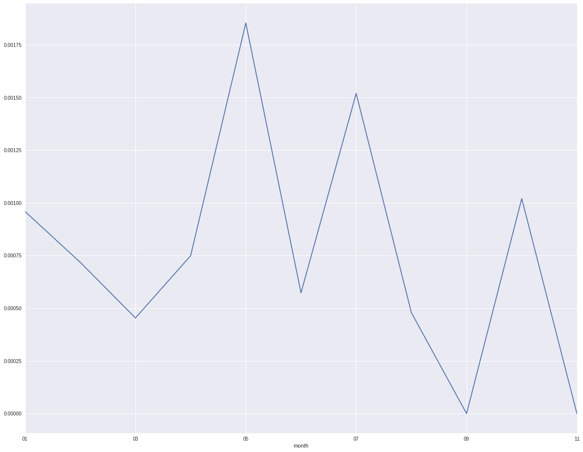
From the plot it shows month 5 and month 7 are higher than the ohter months. There is also period default trend by month.
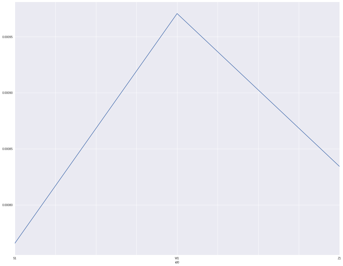
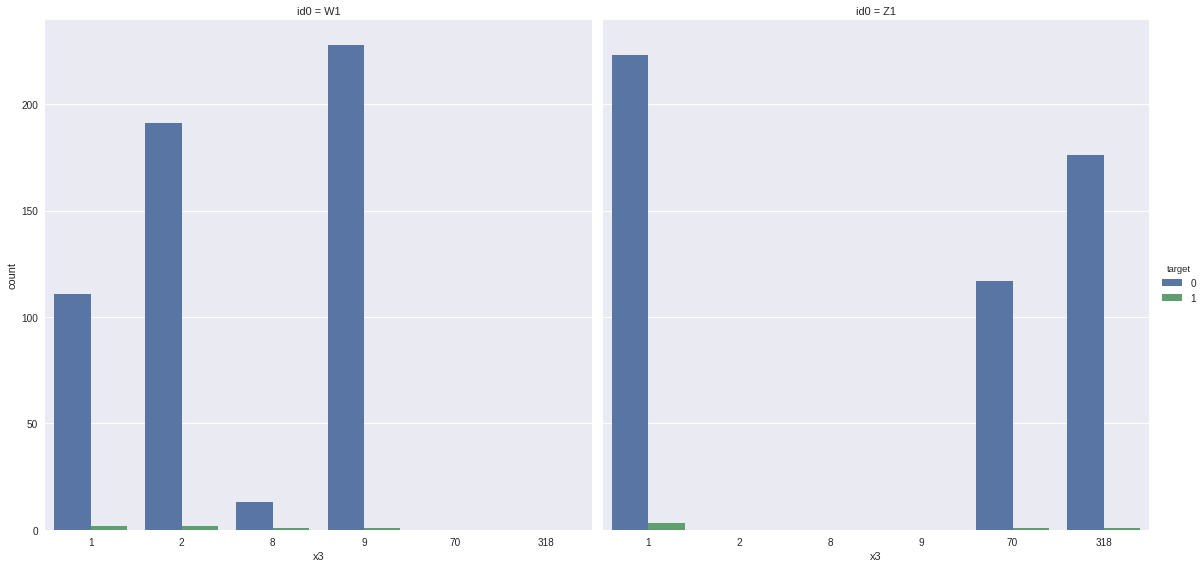
By id it shows w1 has higher default rate then z1. And z1 is higher than s1. Since extracted month and id0 are characters. I will replace them by the log(odds)
indata['month'] = indata.date.map(lambda x: x.split('-')[1])
indata['id0'] = indata.id.map(lambda x: x[:2])
defaults['month'] = defaults.date.map(lambda x: x.split('-')[1])
defaults['id0'] = defaults.id.map(lambda x: x[:2])

def attr_f1(df, x, name):
    print("-"*20 + " this is for x " + x + "-"*20)
    a = df.groupby(x).target.mean().reset_index()
    a.columns = [x, name]
    df = pd.merge(df, a, how = "left", on = x)
    #df.loc[:, name] = np.log((df.loc[:, name] + 1e-8)/(1 - df.loc[:, name] + 1e-8))
    return df

indata = attr_f1(indata, "x2", "a2")
indata = attr_f1(indata, "x3", "a3")
indata = attr_f1(indata, "x4", "a4")
indata = attr_f1(indata, "x5", "a5")
indata = attr_f1(indata, "x7", "a7")
indata = attr_f1(indata, "x8", "a8")
indata = attr_f1(indata, "x9", "a9")
indata = attr_f1(indata, "id0", "id1")
indata = attr_f1(indata, "month", "month0")


defaults = attr_f1(defaults, "x2", "a2")
defaults = attr_f1(defaults, "x3", "a3")
defaults = attr_f1(defaults, "x4", "a4")
defaults = attr_f1(defaults, "x5", "a5")
defaults = attr_f1(defaults, "x7", "a7")
defaults = attr_f1(defaults, "x8", "a8")
defaults = attr_f1(defaults, "x9", "a9")
defaults = attr_f1(defaults, "id0", "id1")
defaults = attr_f1(defaults, "month", "month0")
indata.groupby('month').target.mean().plot()
indata.groupby('id0').target.mean().plot()
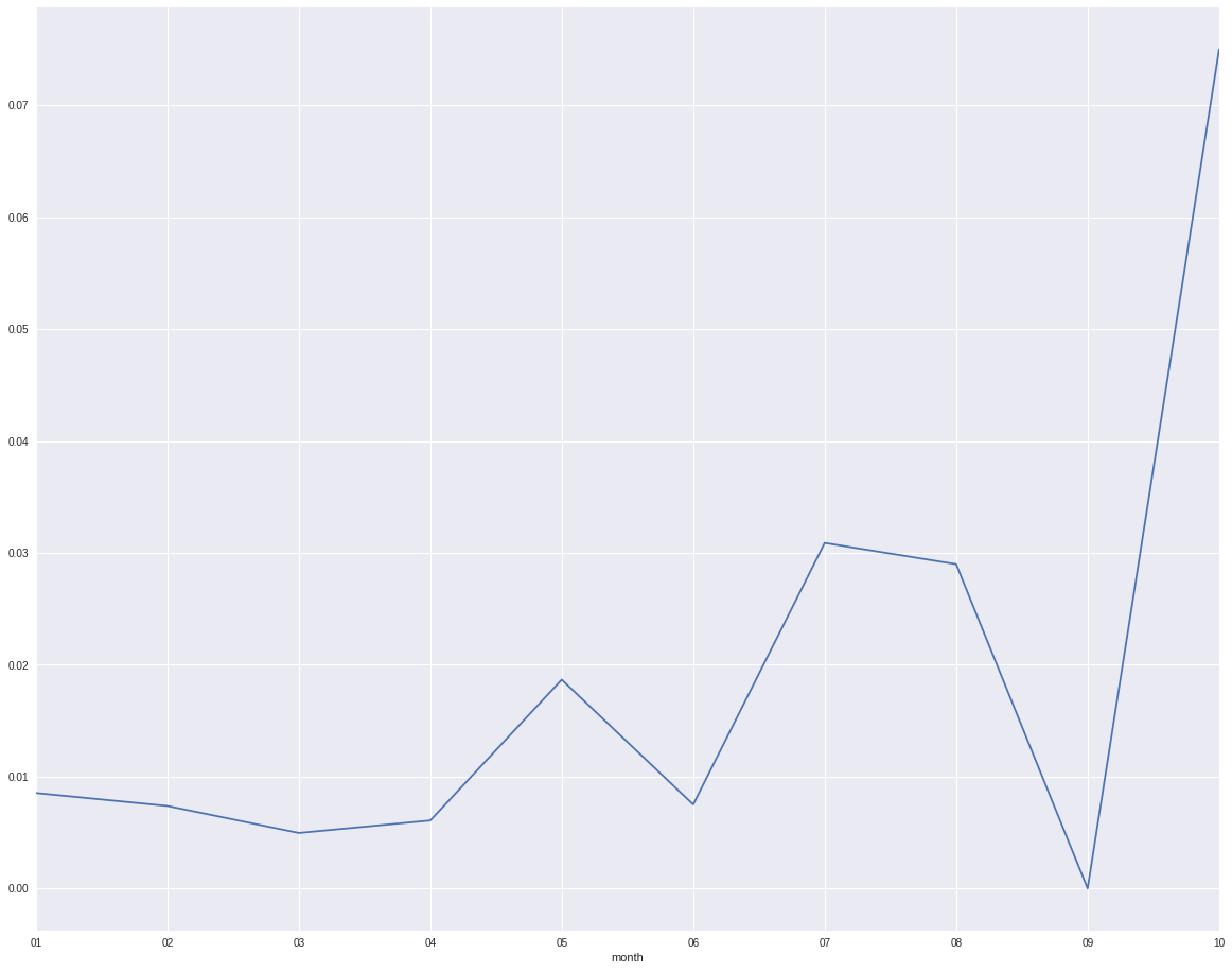
However, when I only look at the defaults data, I will find that month 5 and month 7 are not the highest default month. The trend is not exactly the same as the trend from the full data set.
defaults.groupby('month').target.mean().plot()
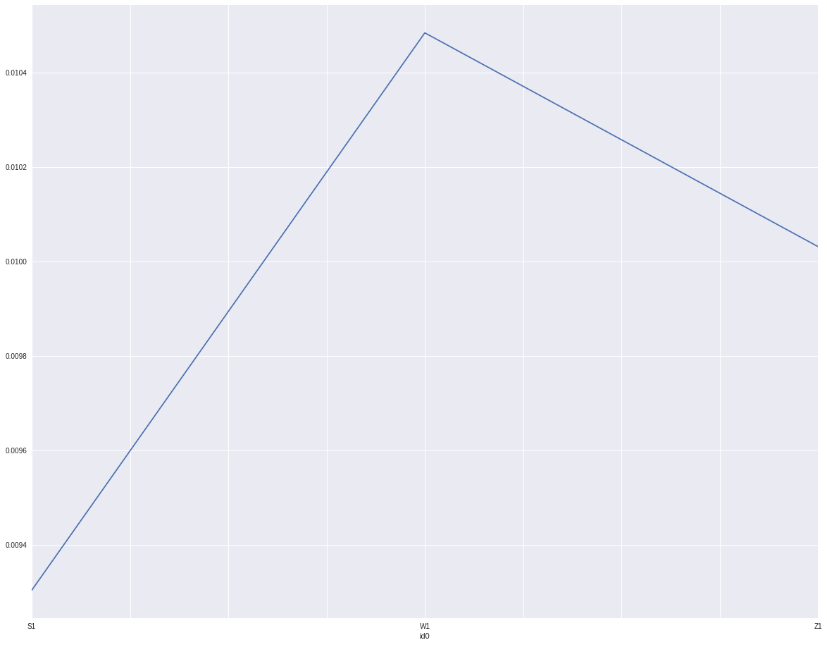
The transformed variable from id still works:
defaults.groupby('id0').target.mean().plot()
sns.factorplot(x = "x3", hue = "target", col = "id0",
               data = defaults[defaults.x3 != 0], kind = "count", size = 8, aspect=1)
2.3. x1 and x6
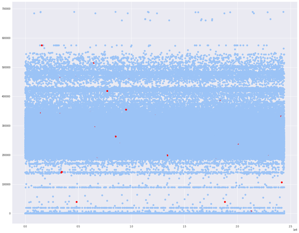
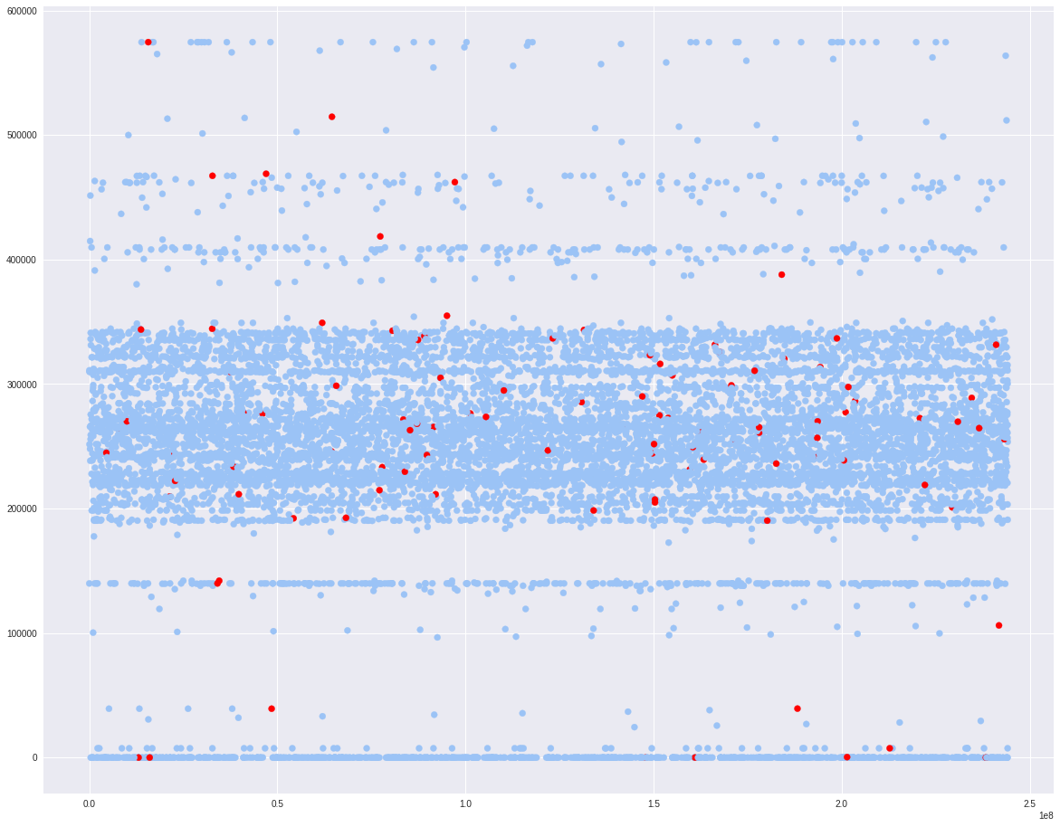
Let us look at the tow continuous variable x1 and x6. I will scatter plot the default rate based on the grids from x1 and x6.
target=0 will be colored as blue and target=1 will be colored as red. It shows most of the x1 are between 200000 to 500000.
fig, ax = plt.subplots()
colors = {0:'#9bc3f6', 1:'#ff0000'}
ax.scatter(indata.x1, indata.x6, c = indata.target.apply(lambda x: colors[x]))
plt.show()
fig, ax = plt.subplots()
colors = {0:'#9bc3f6', 1:'#ff0000'}
ax.scatter(defaults.x1, defaults.x6, c = defaults.target.apply(lambda x: colors[x]))
plt.show()
2.4. Correlation
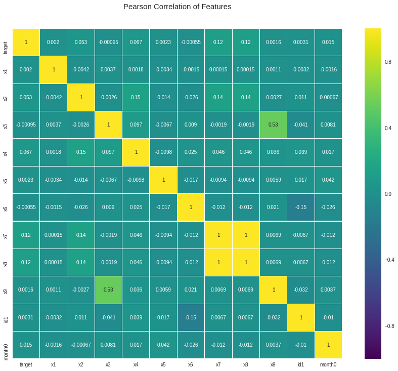
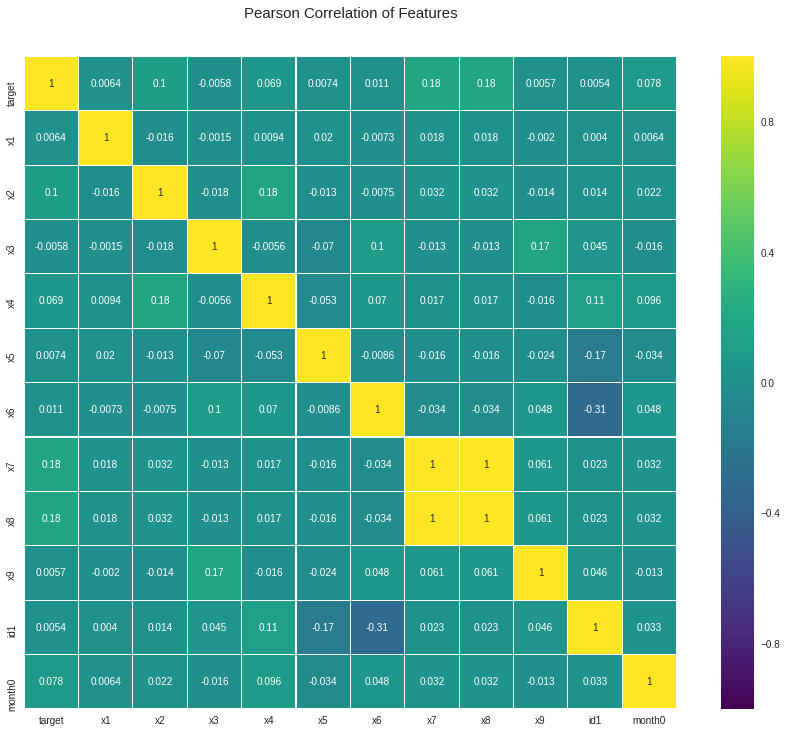
It will be helpful to check the correlation between x and y. Also it is helpful to check the correlation between all the x so that we can know if there is any multicollinearity or not.
We can see there is high correlation between x7 and x8. Alao x9 and 3 has a correlation around 0.53.
cols = ["x1", "x2", "x3", "x4", "x5", "x6", "x7", "x8", "x9", "id1", 'month0']
colormap = plt.cm.viridis
plt.figure(figsize = (16, 12))
plt.title('Pearson Correlation of Features', y = 1.05, size  = 15)
sns.heatmap(indata[["target"] + cols].astype(float).corr(),
            linewidth = 0.1, vmax = 1.0, square = True, cmap = colormap, linecolor = 'white', annot = True)
plt.show()
cols = ["x1", "x2", "x3", "x4", "x5", "x6", "x7", "x8", "x9", "id1", 'month0']
colormap = plt.cm.viridis
plt.figure(figsize = (16, 12))
plt.title('Pearson Correlation of Features', y = 1.05, size  = 15)
sns.heatmap(defaults[["target"] + cols].astype(float).corr(),
            linewidth = 0.1, vmax = 1.0, square = True, cmap = colormap, linecolor = 'white', annot = True)
plt.show()
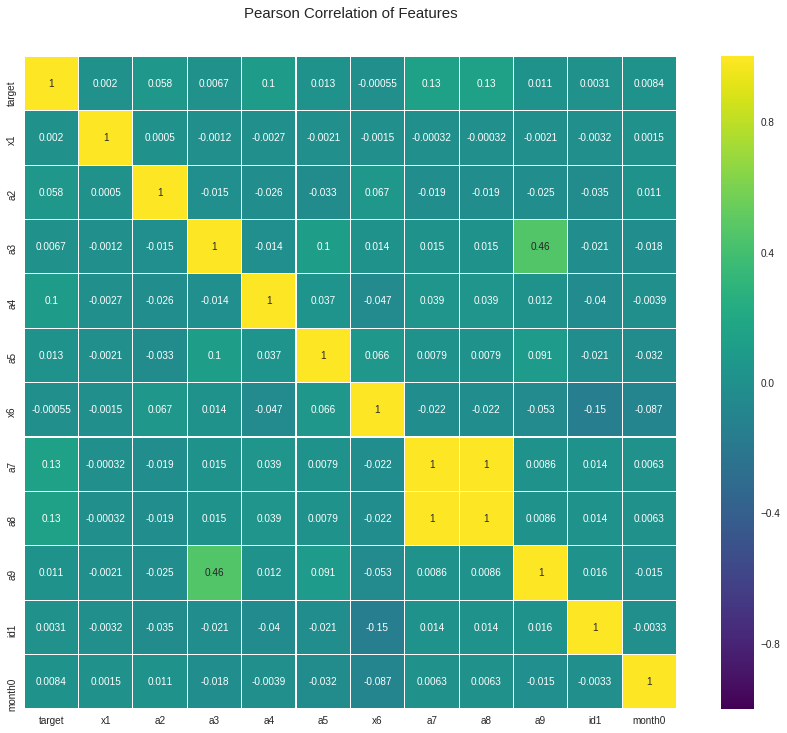
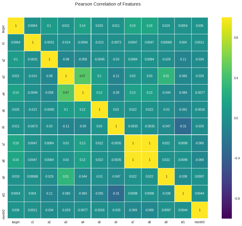
Also, we can check the correlation between y and the transformed values a.
cols = ["x1", "a2", "a3", "a4", "a5", "x6", "a7", "a8", "a9", "id1", 'month0']
colormap = plt.cm.viridis
plt.figure(figsize = (16, 12))
plt.title('Pearson Correlation of Features', y = 1.05, size  = 15)
sns.heatmap(indata[["target"] + cols].astype(float).corr(),
            linewidth = 0.1, vmax = 1.0, square = True, cmap = colormap, linecolor = 'white', annot = True)
plt.show()
cols = ["x1", "a2", "a3", "a4", "a5", "x6", "a7", "a8", "a9", "id1", 'month0']
colormap = plt.cm.viridis
plt.figure(figsize = (16, 12))
plt.title('Pearson Correlation of Features', y = 1.05, size  = 15)
sns.heatmap(defaults[["target"] + cols].astype(float).corr(),
            linewidth = 0.1, vmax = 1.0, square = True, cmap = colormap, linecolor = 'white', annot = True)
plt.show()
3. Model
3.1. Inbalanced Data
Since there are only 106 defaults comparing to 1168 borrowers and 124494 observations, the proportion of target=1 is very low. That is, our data is inbalanced data.
If we used inbalanced data directly to build the model, we might be in trouble because the model will be ignoring the target=1 data if we use accuracy to measure the model performance.
There are some methods to deal with the inbalanced data:
-
oversampling: we repeat the low proportion data to make the proportion of target=1 and target=0 to be close in the oversampled data.
-
downsampling: unlike oversampling to increase the low proportion data, downsampling will try to sample from high proportion(target=1 here) to make the data balanced
-
adjust the low proportion data weight in the algorithm
-
adjust the decision threshold of the output probability to classify
-
adjust the lost function if we want to give more weights on the low proportion data
3.2. Oversampling
Here we will do oversampling:
-
we pick all the 10713 observations of 106 borrowers who has been defaulted. There are 106 target=1 with all the rest 10607 observations having target=0
-
Second we will repeat the 106 positive sample 10607/106 times. After this, in the oversampled data, the ratio of 1 v.s. 0 is about half half.
After the new oversampled data is created, I will split them to training part and validation part.
from sklearn.model_selection import train_test_split, StratifiedShuffleSplit
from sklearn.metrics import log_loss, auc, roc_auc_score

defaults_1 = defaults.query('target == 1')
defaults_0 = defaults.query('target == 0')
defaults_1_rep = pd.concat([defaults_1]*int(np.ceil(len(defaults_0)/len(defaults_1))), ignore_index = True, axis = 0)
defaults_new = pd.concat([defaults_0, defaults_1_rep], ignore_index = True, axis = 0)

cols = ["x1", "a2", "a3", "a4", "a5", "x6", "a7", "a9", "id1", 'month0']
ftrain = defaults_new[cols]
fx_train = defaults_new[cols].values
fy_train = defaults_new[["target"]].values.ravel()
print(np.sum(fy_train))

xtrain, xtest, ytrain, ytest = train_test_split(fx_train, fy_train, test_size = 0.4, random_state = 999)
print(ytest.sum())
10600
4168
3.3. First Model: RandomForestClassifier with growing number of estimatiors
RandomForest is the decision tree based algorithm which builds several decision trees and then combine their output to improve the ability of the model. The method of combining trees is known as ensemble method. Ensembing means combination of weak learners to produce a stronger learner.
3.3.1. Growing RandomForest
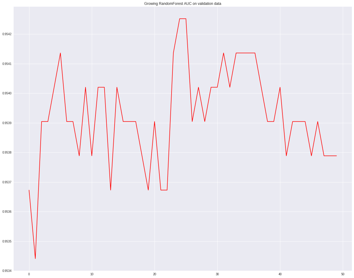
RandomForstClassifier is a combination of many decision trees. In the first example, I will show how the AUC chages based on different number of decision trees. n_estimators is the hyperparameter indicating how many decision trees will be used. We will start from 100 and increase 10 in each loop. Then we will draw the graph of AUC v.s. n_estimators.
Another benifits is we can get the variable importances from the RandomForest output. The variable importances are measured by the total decrease of node impurities from splitting on the variable.
auc = []
growing_rf = RandomForestClassifier(n_estimators=100, criterion='gini', max_depth = 10,
                                    min_samples_leaf = 2, max_features = 'auto',
                                    verbose = 0, n_jobs = -1, warm_start = True, random_state = 168)

for i in range(50):
    growing_rf.fit(xtrain, ytrain)
    growing_rf.n_estimators += 10
    auc.append(roc_auc_score(ytest, growing_rf.predict(xtest)))

_ = plt.plot(auc, '-r')
plt.title("Growing RandomForest AUC on validation data")
Feature importance plot shows that a2 is the most important feature, and a4 is the next most important.
rf_importance = growing_rf.feature_importances_

feature_df = pd.DataFrame({'features': cols, 'RandomForest feature importances': rf_importance})

trace = go.Scatter(y = feature_df['RandomForest feature importances'].values,
                  x = feature_df['features'].values,
                  mode = "markers",
                  marker = dict(sizemode = "diameter",
                               sizeref = 1,
                               size = 25,
                               color = feature_df['RandomForest feature importances'].values,
                               colorscale = "Portland",
                               showscale = True),
                  text = feature_df['features'].values)
data = [trace]

layout = go.Layout(autosize = True,
                  title = "Growing RandomForest Feature Importances",
                  hovermode = "closest",
                  yaxis = dict(title = "Feature Importances",
                              ticklen = 5,
                              gridwidth = 2),
                  showlegend = False)

fig = go.Figure(data = data, layout = layout)

py.iplot(fig, filename = 'scatter2010')
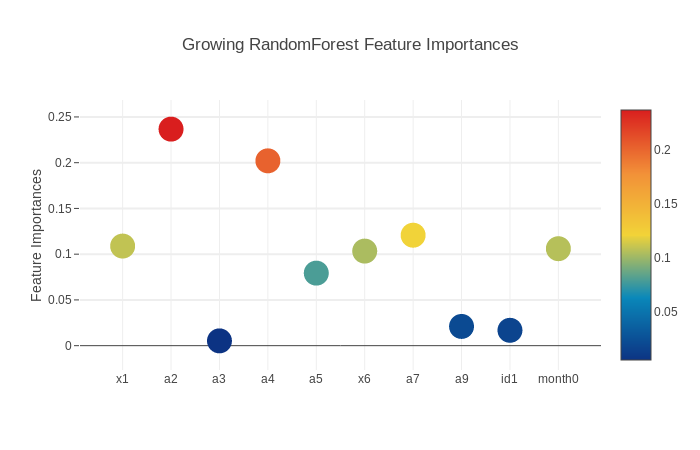
Finally we will apply the built RandomForestClassifier on the original data set. We will get 31 defaults predicted correctly. There are 75 defaults are wrongly predicted as non-defaults. There are also 10 non-defaults are predicted as defaults.
This result also show accuracy is not a good measure here as mentioned above because there are 124378 non-defaults are predicted correctly. So the overall accuracy is very high.
print(confusion_matrix(indata.target, growing_rf.predict(indata[cols])))
[[124384      4]
 [    86     20]]
3.4. GridSearch Hyperparameters
RandomForestClassifier have several hyperparameters to choose. n_estimator will enable you to choose how many decision trees will be used. max_depth will decide how deep the decision tree will be. min_samples_leaf is the minimum number of samples required to be at a leaf node.
We will test the combination of these hyperparameters and let the data decide which hyperparameter is the best. To do that, we first need to define the scoring function which will be the rule to select hyperparameters. From above the main issue here is we are likely to make type 1 and type 2 errors. So I will define a function to minimize the type 1 and type 2 predictions.
from sklearn.grid_search import GridSearchCV
from sklearn.metrics import make_scorer

def myscoring(ground_truth, predictions):
    cmatrix = confusion_matrix(ground_truth, predictions)
    fp = cmatrix[0, 1]
    fn = cmatrix[1, 0]
    return  fn + fp

my_score = make_scorer(myscoring, greater_is_better = False)
estimator = RandomForestClassifier(random_state=0)

rf_tuned_parameters = {"max_depth": [2, 5, 10, 20, 50, 100], 'n_estimators': [20, 50, 100, 200],
                       'min_samples_leaf': [2, 4, 10, 20]}

cv_grid = GridSearchCV(estimator, param_grid = rf_tuned_parameters, scoring = my_score)
cv_grid.fit(xtrain, ytrain)

best_parameters = cv_grid.best_estimator_.get_params()

for param_name in sorted(rf_tuned_parameters.keys()):
    print("\t%s: %r" % (param_name, best_parameters[param_name]))
pred1 = cv_grid.predict(xtest)
print("confustion matrix on validation data: " + str(confusion_matrix(ytest, pred1)))
    max_depth: 20
    min_samples_leaf: 2
    n_estimators: 100
confustion matrix on validation data: [[4259   56]
 [   0 4168]]
pred_full = cv_grid.predict(indata[cols])
print(confusion_matrix(indata.target, pred_full))
[[124384      4]
 [    88     18]]
3.5. ExtraTreeClassifier, AdaboostClassifier, GradientBoostingClassifier, LinearSVC, Logistic Regression
Next I will build some other classification learners. Then these models will be combined together as input for another model. It is like a new ensembling model is created.
Each classifier has its own hyperparameters. It is better to grad search for finetuning hyperparameters and find the best hyperparameters. But that will take longer time to do. To save time I assigned the hyperparameter directly.
The modeling data(oversampled data) will be split into 5 folders. Each time 4 folders data will be used to train a model and the left 1 folder will be used for test data.
3.5.1. Build Model
ntrain = fx_train.shape[0]
nfolds = 5
seed = 888
kf = KFold(ntrain, n_folds=nfolds, random_state=seed)

class SklearnClassifier(object):
    def __init__(self, clf, seed = 999, params = None):
        params['random_state'] = seed
        self.clf = clf(**params)

    def fit(self, x_train, y_train):
        self.clf.fit(x_train, y_train)

    def predict(self, x):
        return self.clf.predict(x)

    def feature_importances(self, x, y):
        return self.clf.fit(x, y).feature_importances_

def get_oof(clf, x_train, y_train):
    oof_train = np.zeros((ntrain, ))
    for i, (train_index, test_index) in enumerate(kf):
        x_tr = x_train[train_index]
        y_tr = y_train[train_index]
        x_te = x_train[test_index]
        y_te = x_train[test_index]
        clf.fit(x_tr, y_tr)
        oof_train[test_index] = clf.predict(x_te)
    full_predict = clf.predict(indata[cols]).reshape(-1, 1)
    return (oof_train.reshape(-1, 1), full_predict)

# random forest parameters
rf_params = {'n_jobs': -1,
            'n_estimators': 50,
            'warm_start': True,
            'max_depth': 50,
            'min_samples_leaf':2,
            'max_features': 'sqrt',
            'verbose':0}

# extra tree parameters
et_params = {'n_jobs': -1,
            'n_estimators': 100,
            'max_depth': 50,
            'min_samples_leaf': 2,
            'verbose':0}

# adaboost parameters
ada_params = {'n_estimators': 100,
             'learning_rate': 0.75}

# gradient boosting parameters
gb_params = {'n_estimators': 100,
            'max_features': 0.5,
            'max_depth': 50,
            'min_samples_leaf':2,
            'verbose':0}

# LinearSVC parameters
svc_params = {'C': 0.25}
rf = SklearnClassifier(clf = RandomForestClassifier, seed = seed, params = rf_params)
et = SklearnClassifier(clf = ExtraTreesClassifier, seed = seed, params = et_params)
ada = SklearnClassifier(clf = AdaBoostClassifier, seed = seed, params = ada_params)
gb = SklearnClassifier(clf = GradientBoostingClassifier, seed = seed, params = gb_params)
svc = SklearnClassifier(clf = LinearSVC, seed = seed, params = svc_params)
from datetime import datetime
startt = datetime.now()

(rf_oof_train, rf_oof_full) = get_oof(rf, fx_train, fy_train)  # 0:00:02.194219
(et_oof_train, et_oof_full) = get_oof(et, fx_train, fy_train)  # 0:00:05.207521
(ada_oof_train,  ada_oof_full) = get_oof(ada, fx_train, fy_train) # 0:00:27.385738
(gb_oof_train, gb_oof_full) = get_oof(gb, fx_train, fy_train)  # 0:00:16.449645
# SVM usually takes too long time to run, use LinearSVC
#https://stackoverflow.com/questions/40077432/scikit-learn-svm-svc-is-extremely-slow
(svc_oof_train, svc_oof_full) = get_oof(svc, fx_train, fy_train)

endt = datetime.now()
print(endt - startt)
0:00:30.987350
3.5.2. Feature Importances
Next we will get the feature importances and plot them. SVM does not have feature importances because it depends on the boundary data points(supporting vectors) on the splitting surface.
rf_features = rf.feature_importances(fx_train, fy_train)
et_features = et.feature_importances(fx_train, fy_train)
ada_features = ada.feature_importances(fx_train, fy_train)
gb_features = gb.feature_importances(fx_train, fy_train)

feature_dataframe = pd.DataFrame({'features':cols,
                                 'Random Forest feature importances': rf_features,
                                 'AdaBoost feature importances': ada_features,
                                 'Gradient Boost feature importances': gb_features,
                                 'Extra trees feature importances': et_features})
def scatter_plot(picked_feature_name = 'Random Forest feature importances'):
    trace = go.Scatter(y = feature_dataframe[picked_feature_name].values,
                      x = feature_dataframe['features'].values,
                      mode = "markers",
                      marker = dict(sizemode = "diameter",
                                   sizeref = 1,
                                   size = 25,
                                   color = feature_dataframe[picked_feature_name].values,
                                   colorscale = "Portland",
                                   showscale = True),
                      text = feature_dataframe['features'].values)
    data = [trace]

    layout = go.Layout(autosize = True,
                      title = picked_feature_name,
                      hovermode = "closest",
                      yaxis = dict(title = "Feature Importances",
                                  ticklen = 5,
                                  gridwidth = 2),
                      showlegend = False)

    fig = go.Figure(data = data, layout = layout)

    py.iplot(fig, filename = 'scatter2010')
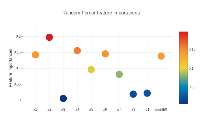
3.5.2.1. RandomForestClassifier Feature Importances
scatter_plot(picked_feature_name = 'Random Forest feature importances')
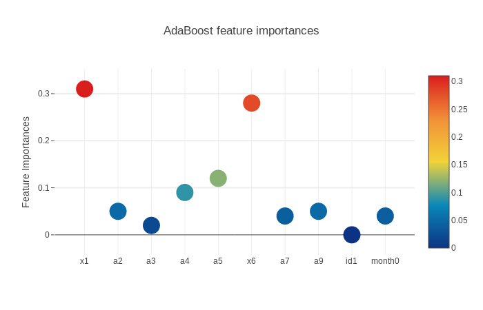
3.5.2.2. AdaBoost Feature Importances
scatter_plot(picked_feature_name = 'AdaBoost feature importances')
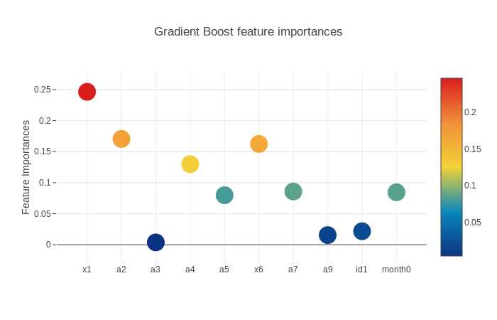
3.5.2.3. Gradient Boost Feature Importances
scatter_plot(picked_feature_name = 'Gradient Boost feature importances')
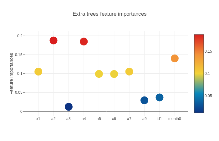
3.5.2.4. Extra trees Feature Importances
scatter_plot(picked_feature_name = 'Extra trees feature importances')
3.6. XGBoost
Finally we will build another model with inputs from the output of the previous models. (This is a little like multi-layers neural network which use previous layers output as current layer input).
This time we will XGBoost to build the model. XGBoost is known for boosted tree learners. It optimizes large scale boosted tree.
base_pred = pd.DataFrame({'randomforest': rf_oof_train.ravel(),
                                'extratree': et_oof_train.ravel(),
                                'adaboost': ada_oof_train.ravel(),
                                'gradientboost': gb_oof_train.ravel(),
                                'linearsvc': svc_oof_train.ravel()})
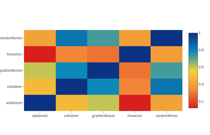
The correlation of the output from the previous model output is given below. We can see the correlation is not very high so we can safely use these output as input for XGBoost model.
data = [
    go.Heatmap(z = base_pred.astype(float).corr().values,
               x = base_pred.columns.values,
               y = base_pred.columns.values,
               colorscale = "Portland",
               showscale = True,
               reversescale = True
              )
]
py.iplot(data, filename = "labelled-Heatmap")
xgb_x_train = np.concatenate((et_oof_train, rf_oof_train, ada_oof_train, gb_oof_train, svc_oof_train), axis = 1)
xgb_y_train = fy_train

import xgboost as xgb

gbm = xgb.XGBClassifier(
    n_estimators = 200,
    max_depth = 50,
    min_child_weight = 2,
    gamma = 0.6,
    subsample = 0.8,
    colsample_bytree = 0.8,
    objective = "binary:logistic",
    nthread = -1,
    scale_pos_weight = 1
).fit(xgb_x_train, xgb_y_train)
confusion_matrix(xgb_y_train, gbm.predict(xgb_x_train))
array([[10267,   340],
       [    0, 10600]])
GridSearch for All
def gscv(estimator, tuned_parameters):
    cv_grid = GridSearchCV(estimator, param_grid = tuned_parameters, scoring = my_score)
    cv_grid.fit(xtrain, ytrain)

    best_parameters = cv_grid.best_estimator_.get_params()

    for param_name in sorted(tuned_parameters.keys()):
        print("\t%s: %r" % (param_name, best_parameters[param_name]))
    pred1 = cv_grid.predict(xtest)
    print("confustion matrix on validation data: " + str(confusion_matrix(ytest, pred1)))
    pred_full = cv_grid.predict(indata[cols])
    print("confustion matrix on validation data: " + str(confusion_matrix(indata.target, pred_full)))
    return pred_full
rf_tuned_parameters = {"max_depth": [2, 5, 10, 20, 50, 100], 'n_estimators': [20, 50, 100, 200],
                           'min_samples_leaf': [2, 4, 10, 20]}
rf_estimator = RandomForestClassifier(random_state=0)
rf_out = gscv(rf_estimator, rf_tuned_parameters)
max_depth: 20
min_samples_leaf: 2
n_estimators: 100

confustion matrix on validation data: [[4259   56] [   0 4168]]
confustion matrix on validation data: [[124384      4] [    88     18]]
et_tuned_parameters = {"max_depth": [2, 5, 10, 20, 50, 100], 'n_estimators': [20, 50, 100, 200],
                           'min_samples_leaf': [2, 4, 10, 20]}
et_estimator = ExtraTreesClassifier(random_state=0)
et_out = gscv(et_estimator, et_tuned_parameters)
max_depth: 50
min_samples_leaf: 2
n_estimators: 200

confustion matrix on validation data: [[4241   74] [   0 4168]]
confustion matrix on validation data: [[124382      6] [    82     24]]
ada_tuned_parameters = {'n_estimators': [20, 50, 100, 200], 'learning_rate': [0.2, 0.5, 1, 2, 5]}
ada_estimator = AdaBoostClassifier(random_state=0)
ada_out = gscv(ada_estimator, ada_tuned_parameters)
learning_rate: 1
n_estimators: 200

confustion matrix on validation data: [[4026  289] [ 151 4017]]
confustion matrix on validation data: [[124388      0] [   105      1]]
gb_tuned_parameters = {"max_depth": [2, 5, 10, 20, 50, 100], 'n_estimators': [20, 50, 100, 200],
                           'min_samples_leaf': [2, 4, 10, 20]}
gb_estimator = GradientBoostingClassifier(random_state=0)
gb_out = gscv(gb_estimator, gb_tuned_parameters)
max_depth: 10
min_samples_leaf: 20
n_estimators: 200

confustion matrix on validation data: [[4287   28] [   0 4168]]
confustion matrix on validation data: [[124386      2] [    77     29]]
svc_tuned_parameters = {"C": [0.2, 0.5, 1, 2]}
svc_estimator = LinearSVC(random_state=0)
svc_out = gscv(svc_estimator, svc_tuned_parameters)
C: 0.2

confustion matrix on validation data: [[4315    0] [4168    0]]
confustion matrix on validation data: [[124388      0] [   106      0]]
xgb_x_train_ = np.concatenate((rf_out.reshape(-1, 1), et_out.reshape(-1, 1),
                               ada_out.reshape(-1, 1), gb_out.reshape(-1, 1),
                               svc_out.reshape(-1, 1)), axis = 1)
xgb_y_train_ = indata.target

gbm = xgb.XGBClassifier(
    n_estimators = 200,
    max_depth = 50,
    min_child_weight = 2,
    gamma = 0.6,
    subsample = 0.8,
    colsample_bytree = 0.8,
    objective = "binary:logistic",
    nthread = -1,
    scale_pos_weight = 1
).fit(xgb_x_train_, xgb_y_train_)
print(confusion_matrix(indata.target, gbm.predict(xgb_x_train_)))
[[124386     2]
 [    60     46]]