If we have a function \(f\), and the objective is to find the point value that can maximize the value of the function. For example, when training DNN, what learning rate or other hyperparameters should we choose to make the loss function as small as possible. Another very practical example: in the allocation of advertisements, when the shopper input a query, the system will propose the corresponding possible advertisements for the allocation system to find the best one to show. Which advertisement will be displayed to the shopper in the end? This is related to many factors, such as the relevance of the advertisement to the query, the click-through rate of the advertisement, the placement of the advertisement, the bid price of the advertisement, and so on. According to these, we will get a comprehensive function, the function \(f\) is the return of all shopper query's potential advertisements. Our topic is to maximize this return, while ensuring that advertising does not affect the shopper's shopping experience.
Because \(f\) is very complicated, this problem is usually difficult to solve directly (for example, it has many factors) or very expensive (for example, it takes a lot of time to try all learning rates, considering it is continuous) or because of many constraints, leading to \(f\) There is no explicit expression.
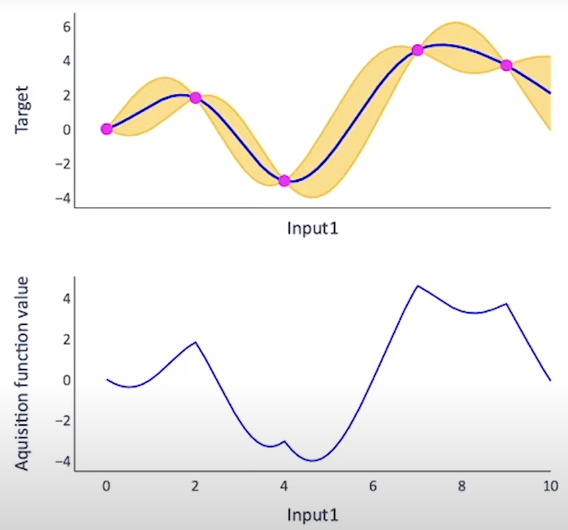
What should we do at this time? In the previous blog, we introduced the construction of a Gaussian process regression based on the limited observation points to surrogate the real \(f\) and the uncertainty.
Acquisition function
Now we need to think about how to get more observation points to tune the Gaussian process and fit the data. The acuqisition function takes the mean and the variance at each point of the GPR function and computes a value that indicates how desirable it is to sample next at this position. A good acquisition function should trade off the exploration and exploitation. With acquisiton function, we don't need the real observations but the point based on the acquisition function (usaally the point that max the acquisition funciton, see details below). With this, the main steps for Bayesian Optimization are:
- Choose a surrogate function (here we use Gaussian process regression) to model the true function \(f\) and define its prior distribution (the kernal function of Gaussian process)
- Based on the given observations, calcualte the posterior distribution through Bayesian formula
- Calculate the acuqisition function \(\alpha(x)\), and determine the next point that maximize the acquisition funciton \(x^* = \mbox{arg max}_x \alpha(x)\)
- Add the new point to the observations and update the posterior
- Repeat the process
1. Objective function
Function \(f\) like a black box usually is not unknown and expensive to evaluate. That is, the explicit expression of \(f\) is unknown and it can only be evaluated based on the test points. Most of the time, only the noisy observations are available.
Usually Gaussian Process (GP) with mean = \(\mu(x)\) and a covariance kernel \(k(x, x')\) is used to surrogate it. That is, for any \(k\) observed points, they have multivariate normal distribution wtih mean = \((\mu(x_0), \ldots, \mu(x_k))\) and covariance matrix \(\Sigma $ with $\Sigma_{ij} = k(x_i, x_j)\). GP surrogate model for \(f\) means \((f(x_1), \ldots, f(x_k))\) is multivariate normal with mean and variance determined by \(\mu(x)\) and \(k(x, x')\).
2. Acquisition Function
| Syntax | Description |
|---|---|
| \(X_n\) | n observed data |
| \(Y_n\) | n observed value |
| \(\hat{y_n^*}\) | max of the n observed value |
| \(y^*, x^*\) | final global max and global optimial point |
Some of the popular acuqisition functions are like:
2.1. Probability Improvement (PI)
PI is to find next \(x_{next}\) s.t. \(f(x)\) will be greater than the maximum from the expirical (denoted with \(y_n^*\)) with a small increse of \(\epsilon\). Here \(f(x)\) is like a random variable from the posterior distribution \(f(x) \sim N(\mu_n(x), \sigma_n(x))\)
- Select the maximum \(\hat{y_n^*} = \mbox{max}_{i \le n}f(x_i)\) based on \(Y_n\)
- For any query point \(x\), put \(x, X_n, Y_n\) into GP to get the function \(f\) at \(f(x)\)'s distribution with mean \(\mu_n(x)\) and \(\sigma_n(x)\), which is normal \(f(x) \sim \mathcal{N}(\mu_n(x), \sigma_n(x))\)
- Get \(x_{next}\) which maximize the PI. \(x_{next} = \mbox{argmax PI}_n(x) = \mbox{argmax P} (f(x) \ge \hat{y_n^*} + \epsilon)\)
- Calc \(f(x_{next})\), update \(X_n, Y_n\) by \(x_{next}, f(x_{next})\) and repeat from step 1.
The parameter \(\epsilon\) is to control exploration and exploitation.
2.2. Expected Improvement (EI)
When use PI to find the next evaluation point \(x_{next}\), it cares about the probability of function value \(f(x) \ge \hat{y_n^*} + \epsilon\). In fact, we should also cares about the distance of function value at evaluation point to the global optimization \(y^8 =f(x^*)\). That is
Since the global optimization point \(y^*\) is unknown, so we use this surrogate to replace the above function
PI cares about the probability while EI cares about how much it is. The detailed steps will be:
- Select the maximum \(\hat{y_n^*} = \mbox{max}_{i \le n}f(x_i)\) based on \(Y_n\)
- For any query point \(x\), put \(x, X_n, Y_n\) into GP to get the function \(f\) at \(f(x)\)'s distribution with mean \(\mu_n(x)\) and \(\sigma_n(x)\), which is normal \(f(x) \sim \mathcal{N}(\mu_n(x), \sigma_n(x))\)
- define \(a^+=\mbox{max}(a, 0)\) and expected distance \(\Delta_n(x) = \mu_n(x) - \hat{y_n^*}\)
- The max expectation improvement point \(x_{next} = \mbox{arg max}_x \mathbb{E}_{f(x) \sim \mathcal{N}(\mu_n(x), \sigma_n(x))}\left(\left(f(x) - \hat{y_n^*} \right)^+\right)\)
- After getting \(x_{next}\), put the new data point \((x_{next}, f(x_{next}))\) into the observations and repeat the processes above.
2.3. Thompson Sampling
In PI and EI, the next point \(x_{next}\) is a single point to maximize some acquisition function. Rather than using one point, it is also possible to draw some points from the posterior distribution such that these points could represent the posterior function. Thompson sampling explots this by drawing such a sample from the posterior distribution and thenchoose the next point \(x_{next}\). Thompson Sampling balances expolration and exploitation in this way:
- Locations with large variance have higher uncertainty. Optimizing such samples will help exploration.
- Samples from current data points have no uncertainty. So if sampling from the surrogate posterior will help exploitation.
2.4. Upper Confidence Bound (UCB)
UCB is the most straightforward method. It is defined as
This setup will favor the region that \(\mu(x^*)\) is large (for exploitation) or regions that \(\sigma(x^*)\) (for exploration) is large. The parameter \(\beta\) is to trade off these two tendencies.
2.5. Others
Some other acquisition funciton are like Knowledge Gradient and Entropy Search.
3. Other surrogate functions
In addition to the Gaussian process, there are some other functions that can work as the surrogate function. For example, random forest is used for sequential model based algorithm; Tree-Parzen estimator works to model the linklihood of the data rather than the posterior.
4. tools
scikit-loptimize provides some examples how to do Bayesian optimization. This Bayesian optimization tool also provides the function to implement the global optimization with Gaussian process. BoTorch provides a scalable tool to implement Bayesian optimization with pyTorch which can leverage GPU to boost the training speed.
5. An simple example
To be continued with BOTorch example.