Before we start Bayesian, we will give a brief introduction of Gaussian Process Regression.
Suppose there are data \((X_i, y_i), i = 1 \cdots n\). If we want to learn the relation between \(X\) and \(y\), we have learned to build a linear regression or a decision tree based model to fit the data. The fitted funciton is like \(y = f(x | \theta)\) where \(\theta\) is the parameter.
Gaussian process regression is infinite number of regression functions. Each function is like one regresson function. All these fitted functions together will not only give the fitted value, but also the variance.
Gaussian process
A Gaussian process is a collection of random variables, where any finite number of these are jointly normal distribution which is defined by: 1) the mean function \(m(x)\) and 2) the covariance function \(k(x, x')\). The function \(\mbox{f}(x) \sim \mbox{GP}(m(x), k(x, x'))\) means
So the Gaussian process can be expressed as
高斯过程的任意有限个样本的联合分布为联合正太分布。
Here for simplify and without loss of generality, we assume the mean is 0. That is,
Gaussian process regression
Suppose we have \(n\) observations \(\left(X_i, y_i=f(X_i)\right), i = 1 \cdots n\), we want to get the prediction given the new data point \(X^*\). Let's denote the \(n\) observations as \(\mathbf{X}=[X_1, X_2, \ldots, X_n]\) and \(\mathbf{f} = [f(X_{1}), f(X_{2}),\ldots, f(X_{n})]\). Based on the property of Gaussian process, the new function value \(f^* = f(X^*)\) is jointly normally distributed with the \(n\) observations
where \(\mathbf{K}[\mathbf{X},\mathbf{X}]\) is a \(n \times n\) matric where the element \((i, j)\) is given by the variance function \(k(X_i, X_j)\), \(\mathbf{K}(\mathbf{X},X^{*})\) is a \(t \times 1\) vector.
Based on the property of joint normal distribution, the conditonal distribution of one element given the rest is also normally distributed with the univariate normal distribution funciton
where
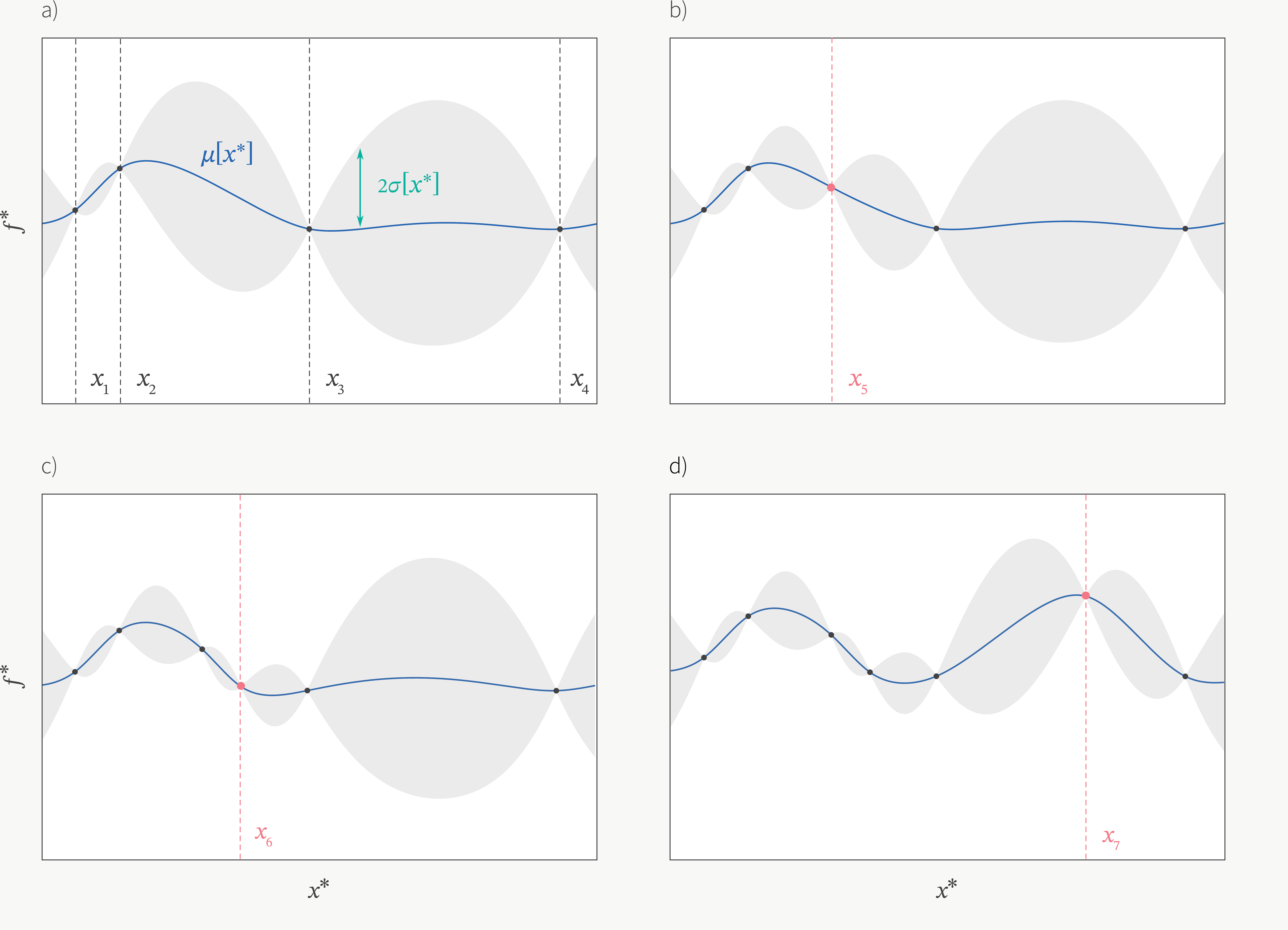
The formula gives the distribution of the prediction \(f(X^*)\) of the new point \(X^*\). As you can see, now \(f(X^*)\) is not a point prediction but a random variable with mean=\(\mu(X^{*})\) and variance=\(\sigma^{2}(X^{*})\). If we want to make a point prediction, then the best prediction will be =\(\mu(X^{*})\). Below is an example of plot of GPR fitted by 4 observations. As the new observations added (for example, \(x_5\)), the uncertainty will go down so the variance will decrease. As more observations onboard, the uncertainty/variance will continue to go down. However, in reality, these observaroins may be expensive to observe or may be hard to get. So the question is, how can we get the new observations to fit the regression? Bayesian Optimization (BO) will provide some ideas about how to get these new data points by maximizing the acquisition function. We will introduce that in next blog.
Next we will give an example of how Gaussian process regression is developed and what it looks like. The code is from this sklearn example.
import numpy as np
import matplotlib.pyplot as plt
import seaborn as sns
plt.rcParams["figure.figsize"] = (32,20)

np.random.seed = 8
X = np.linspace(start = 0, stop=10, num=1000).reshape(-1,1)
y = np.squeeze(X * np.sin(X))

rng = np.random.RandomState(1)
training_indices = rng.choice(np.arange(y.size), size = 6, replace = False)
X_train, y_train = X[training_indices], y[training_indices]

from sklearn.gaussian_process import GaussianProcessRegressor
from sklearn.gaussian_process.kernels import RBF

kernel = 1 * RBF(length_scale=1.0, length_scale_bounds=(1e-2, 1e2))
gaussian_process = GaussianProcessRegressor(kernel=kernel, n_restarts_optimizer = 8)
gaussian_process.fit(X_train, y_train)

gaussian_process.kernel_

mean_prediction, std_prediction = gaussian_process.predict(X, return_std=True)

plt.plot(X, y, label=r"$f(x) = x \sin(x)$", linestyle="dotted")
plt.scatter(X_train, y_train, label="Observations")
plt.plot(X, mean_prediction, label="Mean prediction = $\mu(X)$")
plt.fill_between(
    X.ravel(),
    mean_prediction - 1.96 * std_prediction,
    mean_prediction + 1.96 * std_prediction,
    alpha=0.2,
    label=r"95% confidence interval=$\mu(X) \pm 1.96 \cdot \sigma(X)$",
)

plt.legend()
plt.xlabel("$x$")
plt.ylabel("$f(x)$")
_ = plt.title("Gaussian process regression")
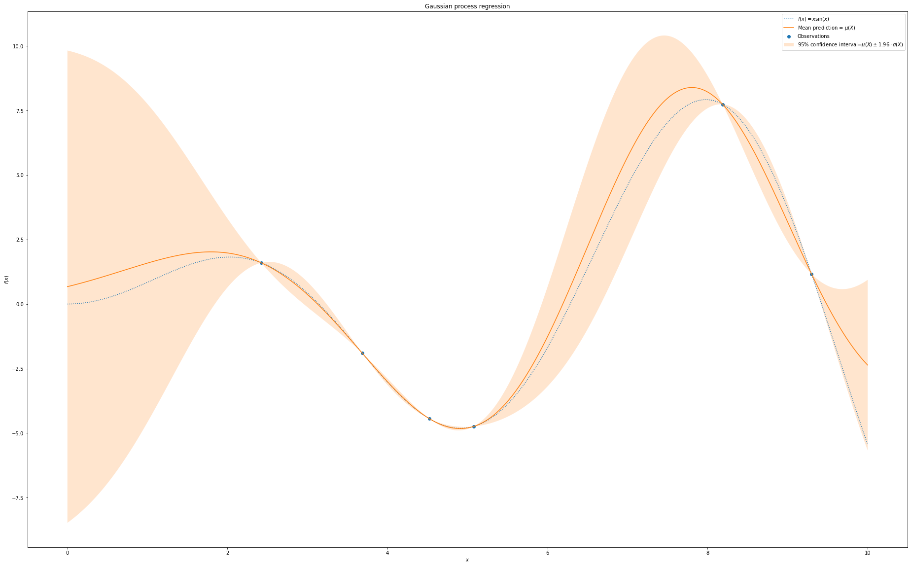 The mean of the Gaussian process regression (red line) is close to the tune function \(y =f(x)= x\cdot \mbox{sin}(x)\). At the points where there is an observation (blue solid dot), the predicted value is exactly the same as the observation. So there is no variance on these points. For the area there is no observatons (the left side), the variance is higher than the area where there are some observations.