Intro
We have two classes of data, the + and the -. Now if there is an unknown point \(\vec{u}\), shall we classify it as + or -?

1) suppose there is a line that can split the + and the -(the dashed line). We project \(\vec{u}\) to the direction perpendicular to the split line, that is, the direction of \(\vec{\omega}\).
Then the decition rule is:
If projection length \(\vec{\omega} \cdot \vec{u} \ge c\), then
+if projection length \(\vec{\omega} \cdot \vec{u} \le c\), then
-
let \(b = -c\), then we have the decision rule is \(\vec{\omega} \cdot \vec{u} + b \ge 0\), then +.
Now we need to find \(\vec{\omega}\) and \(b\) (the parameters to decide the dashed line).
2) Next, for given + and - samples, we want
For math convenience, we define \(y_i\) s.t.
So we have
\(y_i (\vec{\omega} \cdot \vec{x}_ {+} + b) \ge 1\), that is,
\(y_i (\vec{\omega} \cdot \vec{x}_ {+} + b) - 1 \ge 0\) for all
+samples.
Then for the points on the boundary, we have \(y_i (\vec{\omega} \cdot \vec{x}_ {+} + b) - 1 = 0\).
We want the street(distance between two solid line) to be as wide as possible.
The width is \((\vec{x}_ {+} - \vec{x}_ {-})\) projected on the unit direction vector. So the length is

The following are equvalent:
Use Lagrange multipliers,
For \(\vec{x}\) not on the boundary, $\alpha_i $ will be 0. So only the points on the boundary will play role in.
The floowing is an example to show how the boundary points are used in building the linear separater.
To max \(L\), take partial derivatives:
So we have
So, \(\vec{\omega}\) is a linear sum of the vectors \(\sum_ {i} \alpha_ {i} y_ {i} \vec{x}_ {i}\). Since some \(\alpha_ {i}\) will be 0, so, \(\vec{\omega}\) is only some of the vectors sum.
Take partial derivative to \(b\), we have:
So, \(\sum_{i} \alpha_{i} y_{i} = 0\). This is a quadratic optimization problem.
Plug in \(\vec{\omega}\) into \(L\), we will have
Since we have \(\sum_{i} \alpha_{i} y_{i} = 0\), So,
So the max of \(L\) only depends on the pairs of \(\vec{x}_ {i} \cdot \vec{x}_ {j}\).
Plug in \(\vec{\omega}\) into the decision rule, we have
it is also the vector product.
A little more, if the data cannot be splited by a linear line or linear space, what shall we do? Like the data points below, there is no linear method can split the data.
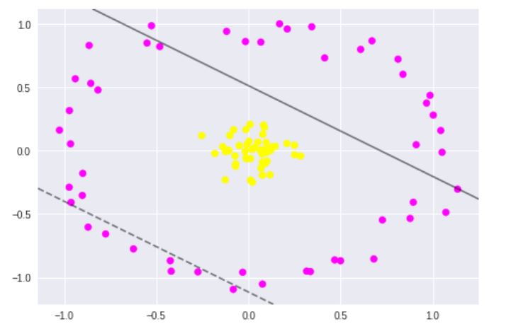
If the data cannot split by a linear line, then we will change vector \(\vec{x}\) to a kernel function \(\phi(\vec{x})\). So we need \(\phi(\vec{x}_ {i}) \cdot \phi(\vec{x}_ {j})\) to max. The kernel is
So what I need is the kernel function \(k\) to map \(\vec{x}_ {i} \vec{x}_ {j}\) to another space.
Choice of \(k\):
1) \(\left(\vec{x}_ {i} \vec{x}_ {j} + 1 \right)^{n}\)
2) \(e^{\frac{||\vec{x}_ {i} - \vec{x}_ {j}||}{\sigma}}\)
Finally, it is an example of kernel function to visualize the second kernel above(rbf kernel):