In the previous blog we introduced diffusion model (DDPM) which is to learn the step (time \(t\)) and the noise function (NN model) by adding Gaussian noise to an image step by step and reversing the process by denosiing from Gaussian noise to an image. Diffusion model is the most important part of Gen AI, however, there are still a few steps from Diffusion model to Gen AI: 1. How to comsume the prompts (instructions to Gen AI to generate a response) in the model? 2. Diffusion model needs huge computaiton as it is running on image pixel directly. To sovle this, latent diffusion model (stable diffusion) was introduced to project the pixel level image to the smaller latent space with perceptual conpression.
What problem Latent Diffusion Models (LDM) solve?
Latent diffusion model (LDM) applies diffusion model on the latent space from encoder rather than the pixel level data. Diffusion model (DDPM) directly adds noise to the image and uses UNet to learn the noise in the denoise step. One challenge here is that it requires a lot of computation with high dimension RGB images in the training step. Also because the noise and denoise needs to be run for many different steps, it makes the computation more expensive and time consumable to run. To solve this problem, the LDM paper (High-Resolution Image Synthesis with Latent Diffusion Models ) proposed an approach to use an encoder (\(\mathcal{E}\)) to convert the image to a latent space \(z\) (which has less dimension than the original image) and and a decoder (\(\mathcal{D}\)) to convert the latent space to image. Diffusion model is then trained on the latent space with better scaling properties because of lower spatial dimension. The reduced complexity also makes it more efficient in image generation from the latent space.
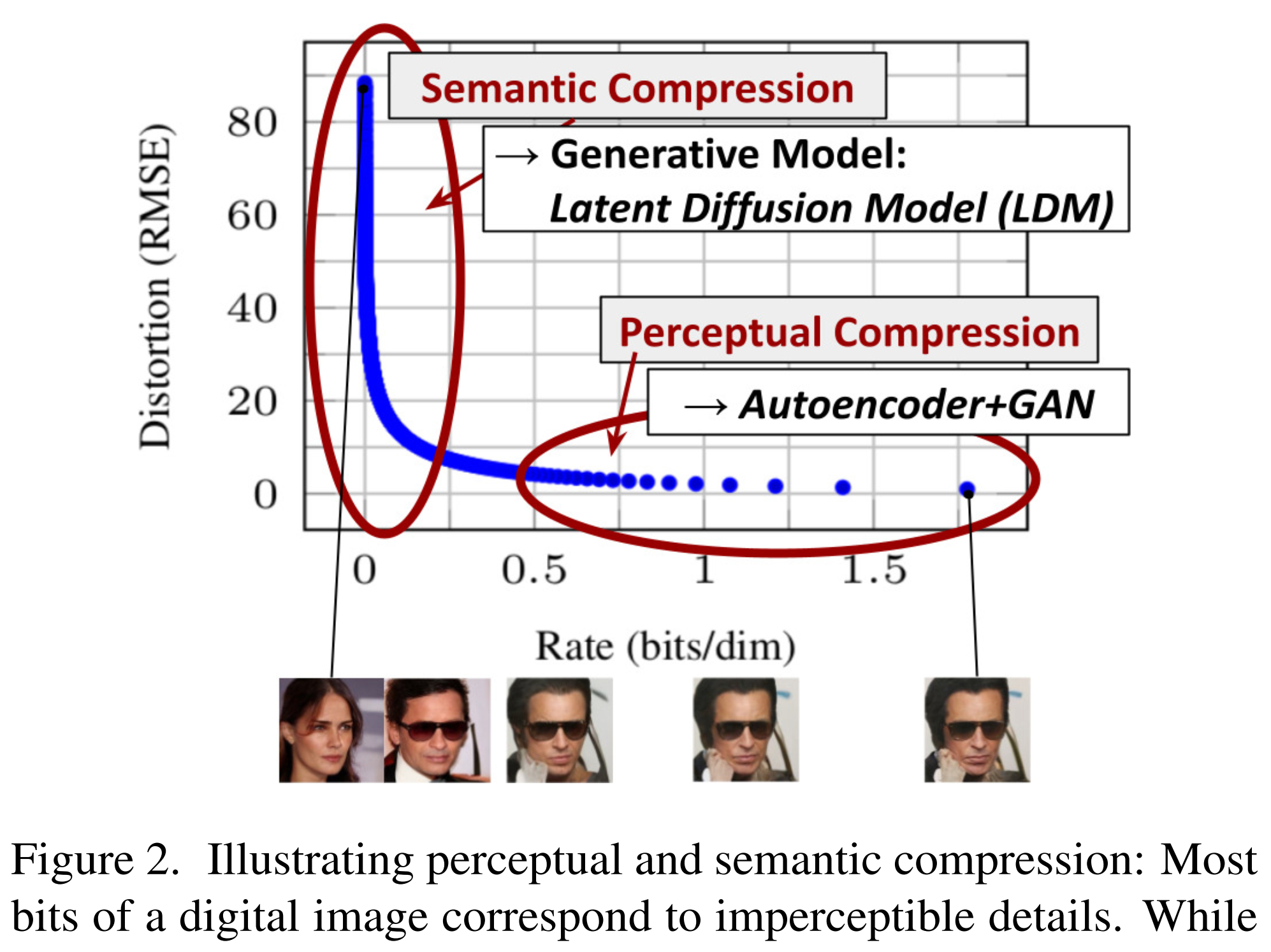
The reason of DP can be done in the latent space is that most bits of a digital image correspond to imperceptible details. After the perceptual compression through the encoder projected to the latent space, most of the perceptual information will still be kept and it only eliminates the imperceptible details. The LDM as a generative model learns the semantic and conceptual composition of the data.
In order to generate images from text prompt \(y\), that is, to predict the probability of latent space \(z\) given prompt \(y\), the authors also design the archtecture of conditional denoising autoencoder \(\epsilon_{\theta}(z_t, t, y)\) which is UNet similar to DM to control the synthesis process with input \(y\) by concating it with the latent space.
How does Latent Diffusion Model work?
1. Perceptual Image Compression
Given an image \(x \in \mathbb{R}^{H × W ×3}\) in RGB space, the encoder \(\mathcal{E}\) encodes \(x\) into a latent representation \(z = \mathcal{E}(x) \in \mathbb{R}^{h×w×c}\), and the decoder \(\mathcal{D}\) reconstructs the image from the latent space with \( \tilde{x} = \mathcal{D}(z) = \mathcal{D}(\mathcal{E}(x))\). The encoder downsamples the image by a factor \(f = H/h = W/w\) where downsampling factors \(f = 2^m\), with \(m \in \mathcal{N}\). For example, if \(m=3\), the original image \(x\) size will be reduced about \(64\) times less.
2. Latent Diffusion Models
Similar to DP model which is to find the \(\epsilon_{\theta}(x_t, t)\) to approximate the error \(\epsilon\) given input image \(x_t\) at step \(t\), latent diffusion model is to find \(\epsilon_{\theta}(z_t, t)\) given the latent space \(z_t\) at step \(t\), where \(\epsilon_{\theta}\) is UNet from 2D convolutional layers. So, starting from an image \(x_t\), LDM includes these steps: 1. Encoder \(\mathcal{E}\) to convert an image \(x_t\) to latent space \(z_t\) 2. Build UNet to learn \(\epsilon_{\theta}(z_t, t)\) 3. Sample from \(P(z)\) and apply the decoder \(\mathcal{D}\) to convert \(z_t\) back to \(x_t\)
3. Conditioning mechanism to generate image from prompt/condition
To generate contents from input like prompt \(y\), the model will not only depends on the time step \(t\), but also the input \(y\), that is the conditional distribution of \(p(z_t | y)\). Accordingly, \(\epsilon_{\theta}(z_t, t)\) is not only the funcion of \(z_t\) and \(t\), but also with input \(y\). That is, \(\epsilon_{\theta}(z_t, t, y)\).
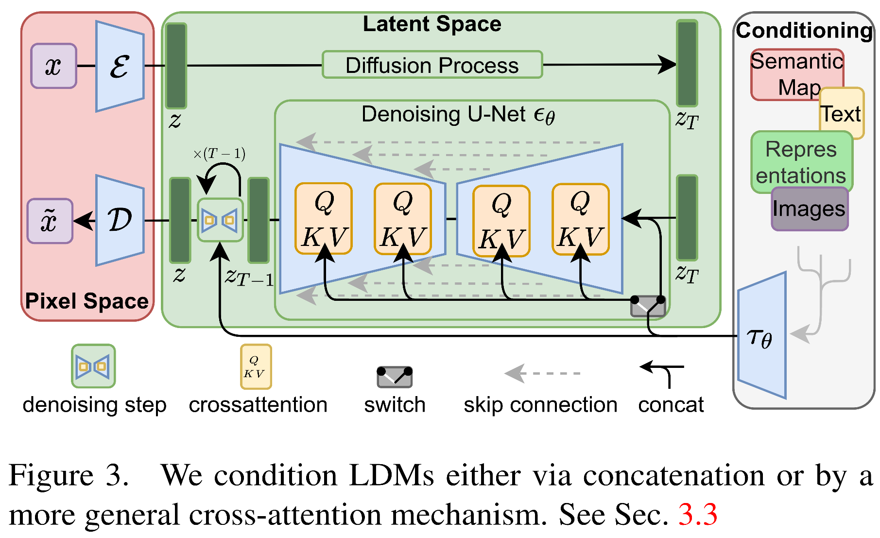
Notations for the figure above:
- \(x\): input of the image. If RGB, its dimension is \(H \times W \times 3\)
- \(\mathcal{E}\) and \(\mathcal{D}\) are the encoder and decoder, where \(\mathcal{E}\) is to project the image to a low dimension space \(z = \mathcal{E}(x)\) which will save the calculation in the later steps, and \(\mathcal{D}\) is to project from the latent space to the image.
- \(\tau_{\theta}\) is the encoder to project the conditional input (e.g., prompt text) to the intermediate space
- \(\epsilon_{\theta}(z_t, t, \tau_{\theta}(y)\) is the conditional denosing autoencoder to denoise from \(z_t\) to \(z_{t-1}\)
The authors develop the attention mechanism to model the cross-attention relationships among the inputs by augmenting the UNet backbone with cross-attention mechanism. The attention is between the condition encoder \(\tau_{\theta}(y)\) and the each intermediate representation layer \(i\) of UNet. To do this, they first build an encoder \(\tau_{\theta}\) to project \(y\) to intermedidate representation \(\tau_{\theta}(y) \in \mathbb{R}^{M \times d_{\tau}}\). The cross-attention is between the \(\tau_{\theta}(y)\) and the projection of the latent space \(\varphi_i(z_t) \in \mathbb{R}^{N \times d_{\epsilon}^i}\) in the UNet with attention defined as
and
Here \( \varphi_{i}(z_t) \in \mathbb{R}^{N \times d_{\epsilon}^i}\) denotes a fattened intermediate representation layer \(i\) of the UNet implementing \(\epsilon_{\theta}\). And \(\tau_{\theta}(y) \in \mathbb{R}^{M \times d_{\tau}}\) is the embedding of the conditinal input. The projection coefficient \(\color{blue}{W_{Q}^{(i)} \in \mathbb{R} ^{d_{\epsilon}^i \times d}}\), \(\color{blue}{W_{K}^{(i)} \in \mathbb{R} ^{d_{\tau} \times d }}\), \(\color{blue}{W_{V}^{(i)} \in \mathbb{R} ^{d_{\tau} \times d }}\).
Note: it seems the notations in the original paper is not correct. In the original paper, the projection is written as
and the size of the weights matrix \(\color{red} {W_{V}^{(i)} \in \mathbb{R} ^{d \times d_{\epsilon}^i} }\), \(\color{red} {W_{Q}^{(i)} \in \mathbb{R} ^{d \times d_{\tau}} }\), \(\color{red} {W_{K}^{(i)} \in \mathbb{R} ^{d \times d_{\tau}} }\) which is not right. Because \(\color{red} { \varphi_{i}(z_t) \in \mathbb{R}^{N \times d_{\epsilon}^i}}\), it is easy to find that the matrix multipicaiton \(\color{red}{Q = W_{Q}^{(i)} \cdot \varphi_{i}(z_t)}\) cannot be conducted if the size is as described in the paper.
Based on this, the conditional LDM is to learn \(\epsilon_{\theta}\) and \(\tau_{\theta}\) from
Code for LDM
1. Encoder-Decoder - project image to latent space and project from latent space to image
In order to avoid arbitrarily high-variance latent spaces, the authors experiment with two different kinds of regularizations. The first variant is KL-reg which imposes a slight KL-penalty towards a standard normal on the learned latent, similar to a VAE. The second is VQ-reg which uses a vector quantization layer within the decoder.
class AutoencoderKL(pl.LightningModule):
    def __init__(self, ddconfig, ...):
        super().__init__()

    ......

    def encode(self, x):
        h = self.encoder(x)
        moments = self.quant_conv(h)
        posterior = DiagonalGaussianDistribution(moments)
        return posterior

    def decode(self, z):
        z = self.post_quant_conv(z)
        dec = self.decoder(z)
        return dec
    ... ...


class VQModel(pl.LightningModule):
    def __init__(self, ddconfig, ...):
        super().__init__()

    ... ...

    def encode(self, x):
        h = self.encoder(x)
        h = self.quant_conv(h)
        quant, emb_loss, info = self.quantize(h)
        return quant, emb_loss, info

    def encode_to_prequant(self, x):
        h = self.encoder(x)
        h = self.quant_conv(h)
        return h

    def decode(self, quant):
        quant = self.post_quant_conv(quant)
        dec = self.decoder(quant)
        return dec

    def decode_code(self, code_b):
        quant_b = self.quantize.embed_code(code_b)
        dec = self.decode(quant_b)
        return dec
    ......
2. Embedding funciton for conditional input from \(y\) to \(\tau_{\theta}(y)\)
Deifferent embedding functions can be applied to convert the conditonal input to the numeric embeding. Like BERT embedding for text, or CLIP embedding for text or image depending on the input data.
class TransformerEmbedder(AbstractEncoder):
    """Some transformer encoder layers"""
    def __init__(self, n_embed, n_layer, vocab_size, max_seq_len=77, device="cuda"):
        super().__init__()
        ...

class BERTEmbedder(AbstractEncoder):
    """Uses the BERT tokenizr model and add some transformer encoder layers"""
    def __init__(self, n_embed, n_layer, vocab_size=30522, max_seq_len=77,
                 device="cuda",use_tokenizer=True, embedding_dropout=0.0):
        super().__init__()
        ...

class FrozenCLIPTextEmbedder(nn.Module):
    """
    Uses the CLIP transformer encoder for text.
    """
    def __init__(self, version='ViT-L/14', device="cuda", max_length=77, n_repeat=1, normalize=True):
        super().__init__()
        ...


class FrozenClipImageEmbedder(nn.Module):
    """
    Uses the CLIP image encoder.
    """
    def __init__(self, **vargs):
        super().__init__()
        ...
3. Attention - attention between K and Q for new V
Query is from the image in DDPM or the latent space is LDM. Key and Value are from the context or the conditions in LDM.
class CrossAttention(nn.Module):
    def __init__(self, query_dim, context_dim=None, heads=8, dim_head=64, dropout=0.):
        super().__init__()
        inner_dim = dim_head * heads
        context_dim = default(context_dim, query_dim)

        self.to_q = nn.Linear(query_dim, inner_dim, bias=False)
        self.to_k = nn.Linear(context_dim, inner_dim, bias=False)
        self.to_v = nn.Linear(context_dim, inner_dim, bias=False)

    def forward(self, x, context=None, mask=None):
        h = self.heads
        q = self.to_q(x)
        context = default(context, x)
        k = self.to_k(context)
        v = self.to_v(context)

        q, k, v = map(lambda t: rearrange(t, 'b n (h d) -> (b h) n d', h=h), (q, k, v))
        sim = einsum('b i d, b j d -> b i j', q, k) * self.scale

        # attention, what we cannot get enough of
        attn = sim.softmax(dim=-1)
        ... ...
4. UNet - learn the noise for step \(t\)
From the code, it shows that for each level of UNet, there is attention block between condition input \(\tau_{\theta}(y)\) and the UNet intermediate representation \(\varphi_i(z_t)\). The attention mechanism is applied in both down sample and up sample levels in UNet.
class UNetModel(nn.Module):
    def __init__(self, ......):
        super().__init__()
        ......

        # param channel_mult: channel multiplier for each level of the UNet.
        for level, mult in enumerate(channel_mult):
            for _ in range(num_res_blocks):
                layers = [ResBlock(...)]

                ch = mult * model_channels
                if ds in attention_resolutions:
                    ......
                    layers.append(
                        AttentionBlock(
                            ch,
                            use_checkpoint=use_checkpoint,
                            num_heads=num_heads,
                            num_head_channels=dim_head,
                            use_new_attention_order=use_new_attention_order,
                        ) if not use_spatial_transformer else SpatialTransformer(
                            ch, num_heads, dim_head, depth=transformer_depth, context_dim=context_dim
                        )
                    )

        # Similar attention is applied in the upsampling steps
5. Loss funcion - loss between the model output and the target, target to optimize
Steps here are: 1. Sample data from the funcion \(q(x)\) 2. Input the sampled data and step \(t\) into the model 3. Calc the MSE loss between the model output and the target
def p_losses(self, x_start, t, noise=None):
    noise = default(noise, lambda: torch.randn_like(x_start))
    x_noisy = self.q_sample(x_start=x_start, t=t, noise=noise)
    model_out = self.model(x_noisy, t)

    loss_dict = {}
    if self.parameterization == "eps":
        target = noise
    elif self.parameterization == "x0":
        target = x_start
    else:
        raise NotImplementedError(f"Paramterization {self.parameterization} not yet supported")

    loss = self.get_loss(model_out, target, mean=False).mean(dim=[1, 2, 3])