Table of Contents
0. Introduction
It is important that credit card companies are able to recognize fraudulent credit card transactions so that customers are not charged for items that they did not purchase.
The datasets contains transactions made by credit cards in September 2013 by european cardholders. This dataset presents transactions that occurred in two days, where we have 492 frauds out of 284,807 transactions. The dataset is highly unbalanced, the positive class (frauds) account for 0.172% of all transactions.
It contains only numerical input variables which are the result of a PCA transformation. Unfortunately, due to confidentiality issues, we cannot provide the original features and more background information about the data. Features V1, V2, ... V28 are the principal components obtained with PCA, the only features which have not been transformed with PCA are 'Time' and 'Amount'. Feature 'Time' contains the seconds elapsed between each transaction and the first transaction in the dataset. The feature 'Amount' is the transaction Amount, this feature can be used for example-dependant cost-senstive learning. Feature 'Class' is the response variable and it takes value 1 in case of fraud and 0 otherwise.
1. Read in data and the libraries
The data is in good shape, that is, there is no missing.
- Data Clean (missing impute / outliers / normalize)
- Feature Engineering (Categorical variables, transformation, correlation analysis)
The provided data is imbalanced, with positive rate around 0.17%.
If we use this data directly to feed the model, the model will prefer to predict all as 0 for a high accuracy of 0 prediction.
import pandas as pd
import numpy as np
import matplotlib.pyplot as plt
import seaborn as sns

from sklearn.preprocessing import StandardScaler, Normalizer, scale
from sklearn.ensemble import RandomForestClassifier, AdaBoostClassifier, GradientBoostingClassifier, ExtraTreesClassifier
from sklearn.svm import SVC, LinearSVC
from sklearn.metrics import confusion_matrix, log_loss, auc, roc_curve, roc_auc_score, recall_score, precision_recall_curve
from sklearn.metrics import make_scorer, precision_score, fbeta_score, f1_score, classification_report
from sklearn.model_selection import cross_val_score, train_test_split, KFold, StratifiedShuffleSplit, GridSearchCV
from sklearn.linear_model import LogisticRegression

%matplotlib inline
plt.rcParams['figure.figsize'] = (16, 9)

seed = 999

creditcard = pd.read_csv('creditcard.csv')
creditcard.columns = [x.lower() for x in creditcard.columns]
creditcard.rename(columns = {'class': 'fraud'}, inplace = True)
Imbalanced data with very low proportion of positive signals
creditcard.fraud.value_counts(dropna = False)
0    284315
1       492
There are 284315 rows (99.8%) with y = 0, and only 492 rows (0.172%) with y = 1. So it is very imbalanced data.
Usually we have these methods to deal with imbalanced data: 1. Collect more data 2. Over-Sampling or Down-Sampling 3. Change the prediction thresholds 4. Assign weights
Here we will do two things:
-
Use LogisticRegression directly to model the data;
-
Over-sampling the data to get a balanced proportion of positive/negative values
Before oversampling, we will first take a random sample as Test data.
creditcard.groupby('fraud').amount.mean()
fraud
0     88.291022
1    122.211321
The reason why I check this:
For non-fraud transactions, the average amount is 88. For fraud transactions, the average amount is 122. So, in average there will be 122 loss for a fraud. Suppose for each transaction, the company can get 2% transaction fee. That is, the average is 88*2% = 1.76.
That means: if we predict a non-fraud as fraud, we might loss 1.76. However, if we miss to detect a fraud transaction, we will loss about 122.
Later I will use this to build a self-defined loss function.
Modeling Part I: Logistic Regression method
Usually for imbalanced data, we can try:
1. Collect more data (which not work here since the data is given)
2. Down-Sampling or Over-Sampling to get balanced samples
3. Change the Thresholds to adjust the prediction
4. Assign class weights for the low rate class
Here we will try 5 different ways and compare their results:
2.1. Do nothing, use original data to model
2.2. Do Over-Sampling, use the over-sampled data to model
2.3. Change the threshold to selected value, rather than using default 0.5
2.4. Assigning sample weights in Logistic Regression
2.5. Change the performance metric, like using ROC, f1-score rather than using accuracy
Since this is Fraud detection question, if we miss predicting a fraud, the credit company will lose a lot. If we miss predicting a normal transaction as Fraud, we can still let the exprt to review the transactions or we can ask the user to verify the transaction. So in this specific case, False Positive will cause more loss than False Negative.
Preprocess data
# 1. Split Test Data Out
creditcard.drop(columns = 'time', inplace = True)

# Normalize the 'amount' column
scaler = StandardScaler()
creditcard['amount'] = scaler.fit_transform(creditcard['amount'].values.reshape(-1, 1))
# creditcard.drop(columns = 'amount', inplace = True)

X = creditcard.iloc[:, :-1]
y = creditcard.iloc[:, -1]
Xtrain, Xtest, ytrain, ytest = train_test_split(X, y, test_size = .33, stratify = y, random_state = seed)
1. Model imbalanced data directly
We will use the imbalanced data directly in logistic regression. That is, the positive rate is about 0.172%. Accuracy is not good since if all predicted as 0, the accuracy for 0 is very high. So, here recall, precision, roc and confusion_matrix are listed to compare model performance.
# 2. If we don't do Over-sampling, what will happen?
X = creditcard.iloc[:, :-1]
y = creditcard.iloc[:, -1]
Xtrain, Xtest, ytrain, ytest = train_test_split(X, y, test_size = .33, stratify = y, random_state = seed)

logitreg_parameters = {'C': np.power(10.0, np.arange(-3, 3))}
logitreg = LogisticRegression(verbose = 3, warm_start = True)
logitreg_grid = GridSearchCV(logitreg, param_grid = logitreg_parameters, scoring = 'roc_auc', n_jobs = 70)

logitreg_grid.fit(Xtrain, ytrain)   # logitreg_grid.best_params_ ; logitreg_grid.best_estimator_

# on OVER-Sampled TRAINing data
print("\n Thre recall score on Training data is:")
print recall_score(ytrain, logitreg_grid.predict(Xtrain))    # 0.58
print("\n Thre precision score on Training data is:")
print precision_score(ytrain, logitreg_grid.predict(Xtrain))   # 0.89

# on the separated TEST data
print("\n Thre recall score on Test data is:")
print recall_score(ytest, logitreg_grid.predict(Xtest))   # 0.58
print("\n Thre precision score on Test data is:")
print precision_score(ytest, logitreg_grid.predict(Xtest))   # 0.86
print("\n Thre Confusion Matrix on Test data is:")
print confusion_matrix(ytest, logitreg_grid.predict(Xtest))
[LibLinear]
 Thre recall score on Training data is:
0.584848484848

 Thre precision score on Training data is:
0.893518518519

 Thre recall score on Test data is:
0.586419753086

 Thre precision score on Test data is:
0.863636363636

 Thre Confusion Matrix on Test data is:
[[93810    15]
 [   67    95]]
Conclusions:
From the output above, we know on the training data, the recall score is 0.58 which means 58 over 100 of the True positive conditions are predicted correctly. And 89 over 100 of the predicted positives are True Positive.
On the Test data, the model performance metric evalued by recall or precision are close to the Training data. There is a precision score of 0.86 on the Test data, which means 86 out of 100 predicted positives are True positives.
From Confusion Matrix, 95 of 162 True Positives are predicted as positives. And of all 110 predicted as positive, 95 of them are True positives.
1.1. Change the Thresholds
ytrain_pred_probas = logitreg_grid.predict_proba(Xtrain)[:, 1]   # prob of predict as 1
fpr, tpr, thresholds = roc_curve(ytrain, ytrain_pred_probas)   # precision_recall_curve
roc = pd.DataFrame({'FPR':fpr,'TPR':tpr,'Thresholds':thresholds})
_ = plt.figure()
plt.plot(roc.FPR, roc.TPR)
plt.axvline(0.1, color = '#00C851', linestyle = '--')
plt.xlabel("FPR")
plt.ylabel("TPR")
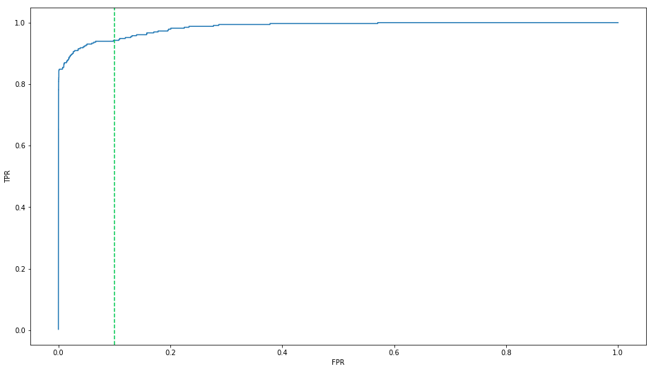
By default, the threshold is 0.5. Since the recall score is low, we shall lower the threshold to get more predicted as Positive. At the same time, more True Negative data will be falsely predicted as Positive. So the Precision score will be lower.
ytest_pred_probas = logitreg_grid.predict_proba(Xtest)[:, 1]
new_threshold = 0.1   # 0.5 is the default value
ytest_pred = (ytest_pred_probas >= new_threshold).astype(int)

print("After change threshold to 0.1, the recall socre on Test data is:")
print recall_score(ytest, ytest_pred)     # 0.827
print("\n After change threshold to 0.1, the precision socre on Test data is:")
print precision_score(ytest, ytest_pred)  # 0.812
print("\nAfter change threshold to 0.1, the Confusion Matrix on Test data is:")
print confusion_matrix(ytest, ytest_pred)
After change threshold to 0.1, the recall socre on Test data is:
0.827160493827

 After change threshold to 0.1, the precision socre on Test data is:
0.812121212121

After change threshold to 0.1, the Confusion Matrix on Test data is:
[[93794    31]
 [   28   134]]
If we lower the threshold to 0.1, we will get recall rate of 0.827. That is, 134 of 162 True Frauds will be detected while only 31 on 165 predicted Frauds are not True Frauds.
If we lower the threshold to 0.01, then the recall score will be 0.91 while the precision score is 0.1.
2. Create Over-sampling data and Fit the model
Since there are much more samples
oversample_ratio = sum(ytrain == 0) / sum(ytrain == 1)  # size to repeat y == 1
# repeat the positive data for X and y
ytrain_pos_oversample = pd.concat([ytrain[ytrain==1]] * oversample_ratio, axis = 0)
Xtrain_pos_oversample = pd.concat([Xtrain.loc[ytrain==1, :]] * oversample_ratio, axis = 0)
# concat the repeated data with the original data together
ytrain_oversample = pd.concat([ytrain, ytrain_pos_oversample], axis = 0).reset_index(drop = True)
Xtrain_oversample = pd.concat([Xtrain, Xtrain_pos_oversample], axis = 0).reset_index(drop = True)

ytrain_oversample.value_counts(dropna = False, normalize = True)   # 50:50

logitreg_parameters = {'C': np.power(10.0, np.arange(-3, 3))}
logitreg = LogisticRegression(verbose = 3, warm_start = True)
logitreg_grid = GridSearchCV(logitreg, param_grid = logitreg_parameters, scoring = 'roc_auc', n_jobs = 70)

logitreg_grid.fit(Xtrain_oversample, ytrain_oversample)   # logitreg_grid.best_params_ ; logitreg_grid.best_estimator_

# on OVER-Sampled TRAINing data
print("\n After Over-Sampling, the recall score on Training data is")
print recall_score(ytrain_oversample, logitreg_grid.predict(Xtrain_oversample))    # 0.918
print("\n After Over-Sampling, the precision score on Training data is")
print precision_score(ytrain_oversample, logitreg_grid.predict(Xtrain_oversample))   # 0.971

# on the separated TEST data
print("\n After Over-Sampling, the recall score on Test data is")
print recall_score(ytest, logitreg_grid.predict(Xtest))   #  0.932
print("\n After Over-Sampling, the precision score on Test data is")
print precision_score(ytest, logitreg_grid.predict(Xtest))   # 0.056
print("\n After Over-Sampling, the Confusion Matrix on Test data is")
print confusion_matrix(ytest, logitreg_grid.predict(Xtest))
[LibLinear]
 After Over-Sampling, the recall score on Training data is
0.918181818182

 After Over-Sampling, the precision score on Training data is
0.971089227494

 After Over-Sampling, the recall score on Test data is
0.932098765432

 After Over-Sampling, the precision score on Test data is
0.0562383612663

 After Over-Sampling, the Confusion Matrix on Test data is
[[91291  2534]
 [   11   151]]
From the output above, we know on the training data, the recall score is 0.918 which means 91.8 over 100 of the True conditions are predicted correctly. And 97 over 100 of the predicted positives are really positive.
However, there is only a precision score of 0.056 on the Test data, which means only 5.6 out of 100 predicted positives are real positives.
From Confusion Matrix, 151 of 162 True Positives are predicted as positives. However, the model predicted 2533 Negative data as Positive.
That is, out model has pretty strong over-fitting.
2.1 Change the Thresholds
ytrain_pred_probas = logitreg_grid.predict_proba(Xtrain)[:, 1]
fpr, tpr, thresholds = roc_curve(ytrain, ytrain_pred_probas)   # precision_recall_curve
roc = pd.DataFrame({'FPR':fpr,'TPR':tpr,'Thresholds':thresholds})

_ = plt.figure()
plt.plot(roc.FPR, roc.TPR)
plt.axvline(0.2, color = '#00C851', linestyle = '--')
plt.xlabel("FPR")
plt.ylabel("TPR")
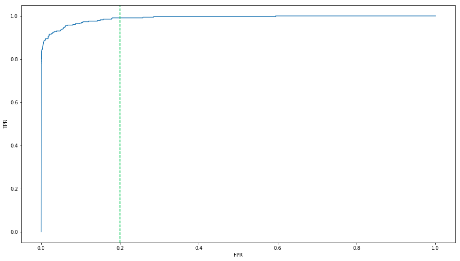
ytest_pred_probas = logitreg_grid.predict_proba(Xtest)[:, 1]
new_threshold = 0.2
ytest_pred = (ytest_pred_probas >= new_threshold).astype(int)

print("After change threshold to 0.2, the recall socre on Test data is:")
print recall_score(ytest, ytest_pred)
print("\n After change threshold to 0.2, the precision socre on Test data is:")
print precision_score(ytest, ytest_pred)
print("\n After change threshold to 0.2, the Confusion Matrix on Test data is:")
print confusion_matrix(ytest, ytest_pred)
After change threshold to 0.2, the recall socre on Test data is:
0.956790123457

 After change threshold to 0.2, the precision socre on Test data is:
0.016130710792

 After change threshold to 0.2, the Confusion Matrix on Test data is:
[[84371  9454]
 [    7   155]]
Conclusion: After over-sampling, the model will have higher recall rate. That is, the model will work better on detect the Frauds from True Frauds. The price we paid is the lower precision rate.
3. Logistic Regression with class_weight
Rather than over-sampling, we can assign more weights to the lower rate class. In fact, if you write out the Likelihood function for Logistic Regression, the Over-Sampling and the assigning more Weights will be equivalent.
positive_weight = sum(ytrain == 0) / sum(ytrain == 1)  # size to repeat y == 1

logitreg_parameters = {'C': np.power(10.0, np.arange(-3, 3))}
logitreg = LogisticRegression(class_weight = {0 : 1, 1 : positive_weight}, verbose = 3, warm_start = True)
logitreg_grid = GridSearchCV(logitreg, param_grid = logitreg_parameters, scoring = 'roc_auc', n_jobs = 70)

logitreg_grid.fit(Xtrain, ytrain)
[LibLinear]


GridSearchCV(cv=None, error_score='raise',
       estimator=LogisticRegression(C=1.0, class_weight={0: 1, 1: 577}, dual=False,
          fit_intercept=True, intercept_scaling=1, max_iter=100,
          multi_class='ovr', n_jobs=1, penalty='l2', random_state=None,
          solver='liblinear', tol=0.0001, verbose=3, warm_start=True),
       fit_params=None, iid=True, n_jobs=70,
       param_grid={'C': array([  1.00000e-03,   1.00000e-02,   1.00000e-01,   1.00000e+00,
         1.00000e+01,   1.00000e+02])},
       pre_dispatch='2*n_jobs', refit=True, return_train_score='warn',
       scoring='roc_auc', verbose=0)
print("\n After assign class_weight, the recall score on Training data is")
print recall_score(ytrain_oversample, logitreg_grid.predict(Xtrain_oversample))    # 0.912
print("\n After assign class_weight, the precision score on Training data is")
print precision_score(ytrain_oversample, logitreg_grid.predict(Xtrain_oversample))   # 0.972

# on the separated TEST data
print("\n After assign class_weight, the recall score on Test data is")
print recall_score(ytest, logitreg_grid.predict(Xtest))   #  0.932
print("\n After assign class_weight, the precision score on Test data is")
print precision_score(ytest, logitreg_grid.predict(Xtest))   # 0.058
print("\n After assign class_weight, the Confusion Matrix on Test data is")
print confusion_matrix(ytest, logitreg_grid.predict(Xtest))
print("\n After assign class_weight, the ROC AUC Score on Test data is")
print roc_auc_score(ytest, logitreg_grid.predict(Xtest))
 After assign class_weight, the recall score on Training data is
0.912121212121

 After assign class_weight, the precision score on Training data is
0.972226568612

 After assign class_weight, the recall score on Test data is
0.932098765432

 After assign class_weight, the precision score on Test data is
0.0581888246628

 After assign class_weight, the Confusion Matrix on Test data is
[[91381  2444]
 [   11   151]]

 After assign class_weight, the ROC AUC Score on Test data is
0.953025135447
If we set up the class weight for the positive as the ratio of non-Fraud / Fraud, we will get the result close to the over-sampling.
So, in summary: This specific data is about fraud detection. So the model should focus on to find the frauds to avoid potential loss for the bank. That is, we should focus on RECALL rate.
- If we use the imbalanced data directly, we will get low performance model since the model prefer to predict to the class with dominated frequency class. The recall rate is 0.58. That is, only 58% of the frauds can be detected by this model.
- To fix that, one way is to do over-sampling or down-sampling. If we use over-sampling, the model performance will be improved a lot. For this specific case, the recall rate on the independent test set will be improved from 0.58 to 0.932
- Another way to improve the model performance is to assign more weights to the low frequency class. Generally speaking, for Logistic Regression, assigning weights is similar to over-sampling, from the likelihood function perspective. The final output results are close too as demonstrated above.