Purpose: achieve the return as much as possible (reduce the regret)

Suppose we want to show the advertisements to the customer and we want to maximize the CTR (click through rate). Let's simplify the situation as there are 3 ads: ad1, ad2 and ad3, the average CTR for them is \(\mu_1 = 0.1, \mu_2 = 0.09, \mu_3=0.0\). If we can show the ads 300 times, then which ad shall we show? In this case, surely we will display ad1 300 times since it is most likely to be clicked by the customer.

But if we not know the value of \(\mu_1, \mu_2, \mu_3\), what shall we do?

Exploration only

Since we don't know which ad will higher ctr, so we may just randomly select an ad to display. In this case, ad1, ad2 and ad3 will be displayed 100 times each. This is called exploration only which means doing it randomly. But it is not good since there is better way: after some random trials (let's say 50 times), we may calcuate the average ctr for each ad, and we may find ad1 has higher ctr than the rest. Then we should display ad1 in the rest 250 times.

class Ad():
    def __init__(self, mu, sigma):
        self.mu = mu
        self.sigma = sigma

    def ctr_sample(self):
        return np.random.normal(self.mu, self.sigma)


def explore(ads, ntotal=300):
    """
    ads is a list of random variables
        each represents the distribution of the corresponding ad
    ntotal: is the total number of trials we can test
    """
    rewards = []
    for _ in range(ntotal):
        rewards.append(random.choice(ads).ctr_sample())
    return rewards

ad1, ad2, ad3 = Ads(0.1, 0.03), Ads(0.09, 0.03), Ads(0.08, 0.03) 

Epsilon-greedy bandit

Rather than choosing the ads randomly, we will try some random choice to explore. After we collect some information, we will exploit to the most highly returned ad.

1. Begin by randomly choosing an ad for each visitor and observing whether it receives a click.
2. As each ad is chosen and the click observed, keep track of the CTR (empirical CTR).
3. Start assigning “most” visitors to your top performing ad by empirical CTR at that point in time, otherwise randomly choose among your other ads.
4. As the empirical CTR changes with more trials, continue updating which ad you assign to most visitors.

The key parameter we decide upon for an epsilon-greedy bandit is \(\epsilon\). \(\epsilon\) manages the exploration / exploitation trade-off by determining what proportion of ads we assign to exploration \(\epsilon\), and exploitation, \(1 - \epsilon\). For example, if \(\epsilon = 0.1\), means 10% of the 300 total trials will be used for exploration (30 times).

Let's denote \(P_t(i)\) as the probability to choose ad \(i\) in the \(t_{th}\) trial, \(K\) as the number of ads, and \(N_t(i)\) is the number of trials for ad \(i\) in the \(t\) trials.

import numpy as np
import matplotlib.pyplot as plt
import seaborn as sns
import random

class EpsilonGreedyBandit():
    def __init__(self, true_ctr, epsilon = 0.1):
        self.epsilon = epsilon
        self.num_ads = len(true_ctr)
        self.ad_ids = np.arange(self.num_ads)
        self.weights = np.full(self.num_ads, 1/ self.num_ads)
        self.clicks = np.zeros(self.num_ads)
        self.trials = np.zeros(self.num_ads)
        self.true_ctr = true_ctr
        self.empirical_ctr = np.zeros(self.num_ads)

    def choose_ad(self):
        """
        Choose ad to display based on the updated weights
        1. Choose the current best ad with prob 1-epislon
        2. Or randomly explore with prob epislon/(num_ads - 1)
        """
        ad = np.random.choice(self.ad_ids, size = 1, p = self.weights)[0]
        return ad

    def click(self, ad):
        """
        Customer click with prob = true_ctr
        """
        click = np.random.binomial(size = 1, n = 1, p=self.true_ctr[ad])[0]
        return click


    def update(self, ad, click):
        """
        For given ad, update the values
        """
        self.clicks[ad] += click
        self.trials[ad] += 1
        self.empirical_ctr[ad] = self.clicks[ad] / self.trials[ad]
        if self.clicks.any():
            self.weights[:] = self.epsilon / (self.num_ads - 1)
            best_ad = np.argmax(self.empirical_ctr)
            self.weights[best_ad] = 1 - self.epsilon

    def run_trial(self):
        ad = self.choose_ad()
        click = self.click(ad)
        self.update(ad, click)


# Run an example

emp_ctr = []
ctr = [0.1, 0.09, 0.08]

for i in range(6):
    egb = EpsilonGreedyBandit(ctr)
    for j in range(10**i):
        egb.run_trial()

    emp_ctr.append(egb.empirical_ctr)

emp_ctr = np.array(emp_ctr)

fig, ax = plt.subplots(figsize=(16, 8))

for i in range(len(ctr)):
    plt.plot(emp_ctr[:, i], label = "CTR for ad" + str(i))
plt.legend()
plt.title('Epsilon Greedy Bandit CTR Simulation')
plt.show()

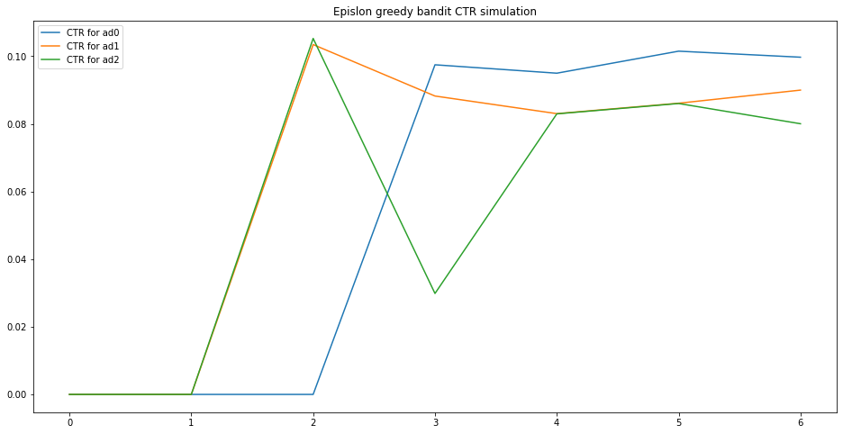As we can see, the empirical CTR will concerge to the true CTR and the best ad will be chosen.

Upper confidence bound (UCB)

In Epsilon-greedy bandit, we only choose the ad based on the empirical_ctr. This might be a little risky since you may lose some information. Let's say there are two ads, after some trials, ad1 has empirical_ctr=0.1, and ad2 has empirical_ctr=0.11. In this case, our algorithm will choose ad2 to exploit since it has higher empirical_ctr. But if ad1 is only shown once, and ad2 has already been shown 20 times. Under this scenario, shall we give ad1 a little more change since it is only being shown 1 time?

UCB is the complement method. In UCB, the best ad is chosen based on who has the highest \(\mbox{empirical_ctr} + \sqrt{{2 ln(t)}/{N_t(i)}}\).

\(N_t(i)\) is the number of trials for ad \(i\) in the \(t\) trials. In the scenario above, ad1 was only shown 1 time, so \(N_t(1) = 1\) and \(N_t(2)=20\) since ad2 was shown 20 times. Because \(N_t(i)\) is in the denominator, as it higher (already shown more time), the corresponding has less likelihood to be selected again unless it has very high empirical_ctr.

Thompson sampling bandits

Thompson sampling bandits (Bayesian bandits) is to chose the action that maximize the expected reward. It aims to tackle the exploration-exploitation trade off in a Bayesian way.

Let denote the action of click or not as a random variable \(X, X=1\) means click and \(0\) means not. If we consider CTR as a parameter \(p\) which is unknown, that is \(P(X=1) = p\). In fact, \(X\) has Bernoulli distribution \(P(X=x|p) = p^x (1-p)^{1-x}\). In this scenario, the conjugate prior for \(p\) is beta distribution \(p \sim Beta(a, b) = p^{a-1} (1-p)^{b-1}\). The posterior distribution is also Beta distribution \(\sim Beta(a+x, b+1-x) = p^{a-1+x} (1-p)^{b-1 + 1-x }\). That is, if the ad is clicked \(x = 1\), so \(a\) will add 1. Otherwise \(b\) will add 1. If we have 10 ads, then we will have 10 posterior beta distributions with their own \(a\) and \(b\). To update the simulation, for each step, we will sample a random value (which is \(p\)) from each of the posterior distribution and pick the ad with the max sampled \(p\) to show.

The general idea is: suppose at time \(t\) (already run \(t\) trials in total), \(N_t(i)\) is the number of trials for ad \(i\) in the \(t\) trials. The posterior probability for ad i is given by the formula above. To do the simulation, we only need these steps:

1. Randomly draw a CTR from each ad’s posterior beta distribution.
2. Choose the ad with the highest drawn CTR.
3. If a click is observed increment \(a\) by 1, otherwise increment \(b\) by 1. (\(\alpha\) and \(\beta\) in the Beta distribution.)

class ThompsonSamplingBandit():
    def __init__(self, true_ctr):
        self.num_ads = len(true_ctr)
        self.ad_ids = np.arange(self.num_ads)
        self.clicks = np.zeros(self.num_ads)
        self.alphas = np.ones(self.num_ads)
        self.betas = np.ones(self.num_ads)
        self.trials = np.zeros(self.num_ads)
        self.true_ctr = true_ctr
        self.empirical_ctr = np.zeros(self.num_ads)

    def choose_ad(self):
        beta_draws = np.zeros(self.num_ads)
        for ad in self.ad_ids:
            draw = np.random.beta(self.alphas[ad], self.betas[ad], size = 1)[0]
            beta_draws[ad] = draw
        best_ad = np.argmax(beta_draws)
        return best_ad

    def click(self, ad):
        click = np.random.binomial(size = 1, n = 1, p = self.true_ctr[ad])[0]
        return click

    def update(self, ad, click):
        self.trials[ad] += 1
        self.clicks[ad] += click
        self.empirical_ctr[ad] = self.clicks[ad] / self.trials[ad]
        if click:
            self.alphas[ad] += 1
        else:
            self.betas[ad] += 1

    def run_trial(self):
        ad = self.choose_ad()
        click = self.click(ad)
        self.update(ad, click)

tsb = ThompsonSamplingBandit(true_ctr = [.2, .15, .1])
for _ in range(200000):
    tsb.run_trial()

print(tsb.empirical_ctr)

# array([0.20028314, 0.14479638, 0.09352518])

emp_ctr = []
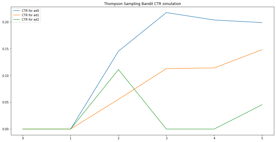
ctr = [0.2, 0.15, 0.08]

for i in range(6):
    egb = ThompsonSamplingBandit(ctr)
    for j in range(10**i):
        egb.run_trial()

    emp_ctr.append(egb.empirical_ctr)

emp_ctr = np.array(emp_ctr)

fig, ax = plt.subplots(figsize=(16, 8))

for i in range(len(ctr)):
    plt.plot(emp_ctr[:, i], label = "CTR for ad" + str(i))
plt.legend()
plt.title('Thompson Sampling Bandit CTR simulation')
plt.show()

However, in reality, \(p\) is not simply a random value, itself maybe a function of different variables / setups. Let’s assume we use logistic regression f to model \(p\). That is, \(p = f(variables, weights)\) and we denote weights as \(w\) which is a vector with \(dim=d\). Now we need to find \(w\) to optimize CTR. The conjugate prior for \(w\) is normal distribution. And the corresponding posterior of \(w\) is also normal distribution. After we observed (x, y), w and the posterior will be updated.

In a more general case, the number of variables and \(w\) of logistic regression may also be random. In this case, we cannot use fixed number of \(dim=d\) priors of normal distribution. We need to extend it to Gaussian processes.

Now we will define the Bayesian Optimization problem.

Objection:

1. output: Objection function \(f\) is continuous
2. Input: complexity depends on dim \(d\)
3. Restriction of \(A\): hyper-rectangle \(\{ x \in \mathbb{R}^d: a_i \le x_i \le b_i \}\) or simplex \(\{ x \in \mathbb{R}^d: \sum_{i} x_i = 1 \}\)
4. \(f\): usually \(f\) is very complicated, it is not linear or convex. It is called black-box.
5. Evaluation: usually there is restriction on the number of trials to evaluate \(f\). derivative-free
6. Target: the target is to find global optimizaion \(x^*\) to max \(f\). It is called global optimization.
7. With these, Bayesian optimization is also called black-box derivative-free global optimization.

It mainly includes two parts: Gaussian Process Regression and Acquisition Function

1. GPR: based on prior and observations to calculate the posterior distribution
2. AF: from the posterior of GPR to get surrogate to find next point to be evaluated

To be continued.