1. What the problem to solve?

When I went back for the Spring Festival, DeepSeek released a new model. For a while, all kinds of media discussed it a lot, almost rising to the height of national destiny. The most important points discussed should be two: the first is the benchmark score comparable to other mainstream models; the second is that the training speed is much faster and uses much less GPU time. However, most of the discussions are prosperous discussions and exciting news, but there is no specific reason why DS is good and how it is good. The first weekend after I came back, I spent the weekend reading the DS V3 paper. The reason why I chose V3 is that R1 is RL and SFT to enhance the reasoning ability of the model. The basic model is still V3, and the DS V3 paper is more detailed. The second part of the article describes what improvements DS has made in the model architecture (science), and the third part describes what improvements have been made in the model training (engineering). Then the two parts talk about pretraining, posttraining and evaluation related things.

2. How to solve?

2.1. Basic Architecture

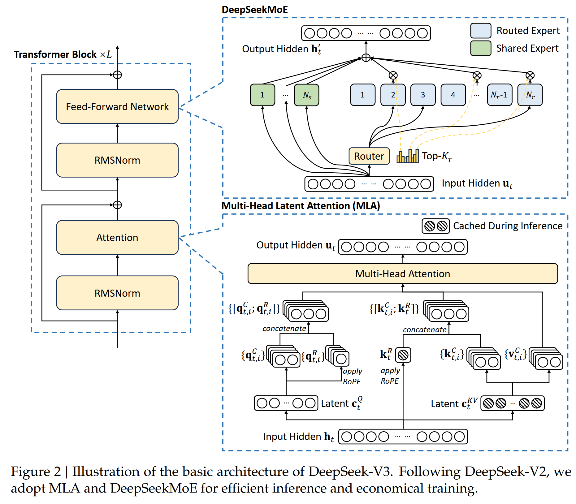
There are two main points in the basic architecture of the model: 1. The original Attention is changed to Multi-head Latent Attention; 2. The original FFN is changed to DeepSeekMoE. The purpose of doing this is to reduce the amount of calculation and reduce the cache data, thereby saving GPU memory. The details are as follows:

DeekSeek Model Architecture

2.1.1. Multi-head latent attention (MLA)

Compared with the attention mechanism introduced in the original Attention model, DS uses the Multi-head latent attention (MLA) architecture. The difference from the original Multi-head attention is that when calculating \(k, q, v\) from \(h_t\), it first reduces the dimension and projects \(h_t \in \mathbb{R}^d\) to a low-dimensional space \(\textcolor{blue}{c_t^{KV} = W^{DKV} h_t}\), and then upgrades the dimension to \(\textcolor{blue}{k_t^C=W^{UK}c_t^{KV}}\); and projects it to a low-dimensional \(\textcolor{blue}{c_t^Q=W^{DQ}h_t}\), and then upgrades the dimension to \(\textcolor{blue}{q_t^C = W^{UQ} c_t^Q}\). In this case, when performing inference, we only need to save low-dimensional \(\textcolor{blue}{c_t^{KV}}\) and \(\textcolor{blue}{c_t^Q}\). For example, the original \(\text{dim}(h_t) = 7168\) is reduced to 4096 dimensions through a dimensionality reduction matrix \(\text{dim}(W^{DKV})=4096 \times 7186\), so the matrix \(\textcolor{blue}{c_t^{KV}}\) that needs to be saved is much smaller. Specifically,

Here \(W^{DKV} \in \mathbb{R}^{d_c \times d}\) is a dimension reduction projection matrix; \(W^{UK}, W^{UV} \in \mathbb{R}^{d_h n_h \times d_c}\) are the corresponding dimension increase matrices of keys and values. When doing inference, only \(\textcolor{blue}{c_t^{KV}}\) and \(\textcolor{blue}{k_t^R}\) are needed, which saves both computation and memory.

For query, the same process is used to reduce the dimension

2.1.2. DeepSeekMoE with Auxiliary-Loss-Free Load Balancing

Basic Architecture of DeepSeekMoE

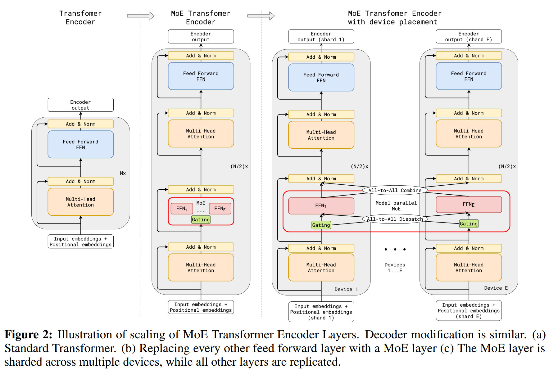
In the 2017 Attention paper, the decoder first calculates Attention and then calculates FFN to predict the final token. In DS, FFN is further changed to MoE. MoE means that the model is composed of a series of Experts. Each Expert can be an MLP, a CNN or other neural network model, or each Expert can be a tansformer encoder/decoder. Each Expert is responsible for learning different data patterns. MoE selects the appropriate Expert through the Gating Network so that different data is sent to the best Expert for processing. When predicting the next token, MoE does not use a certain Expert or all Experts, but selects the Top \(K\) Experts to make predictions. Which \(K\) Experts are selected is determined by a Gating network. Usually \(K \ll N\), so MoE is a sparse network. The first advantage of using MoE is that through more refined divisions, the model has greater flexibility, and different Experts can learn different data. For example, if \(N=16\), \(K=2\), then there are \(C(16, 2)=160\) combinations. If each Expert is split into 4 small Experts, the total number of combinations is \(C(64, 8)=4,426,165,368\). This greatly increases the flexibility of the model. The second benefit is saving computing resources, because only a few Experts need to be activated each time to participate in the calculation, unlike the transformer where all parameters participate in the calculation. In other words, MoE can train a larger model with more parameters, thereby remembering more knowledge, but only a small number of parameters actually participate in the calculation each time. And because each Expert is an independent model with no shared parameters, they can perform calculations in parallel.

MoE Architecture

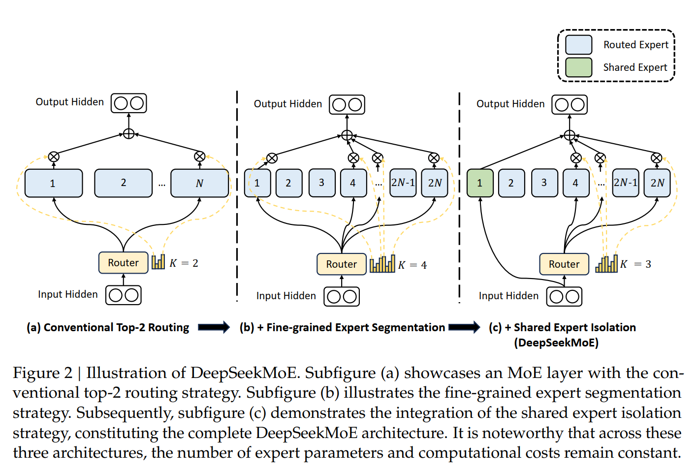
In DS's FFN, DeepSeekMoE goes a step further on the basis of MOE: 1) They further refine the Expert, and then some Experts are used for routing. Specifically, for the routingd Expert, the prediction is only routed to some of these Experts. At the same time, they also have some Experts that are shared Experts, that is, they are used every time when predicting. 2) DS optimizes the selection of Experts and uses affinity scores to select experts. 3) DS's Experts are finer and sparser. This further reduces the computing cost.

DeepSeekMoE Architecture

Assuming that the center of each Expert \(i\) is \(\mathbf{e}_{i}\), first calculate \(\textcolor{blue}{s_{i,t} = \sigma(\mathbf{u}_t^\top \mathbf{e}_i)}\) as the similarity between token \(t\) and Expert \(i\): \(\mathbf{e}_i\) is used as the center vector of Expert \(i\). The dot product is performed with the input \(\mathbf{u}_t\) of the token, and then the affinity of the token to the Expert is calculated through sigmoid, thereby determining whether the token is routed to the Expert.

\(g^{\prime}_{i,t}\) is the gating value of Expert \(i\). Based on the value of \(s_{i,t}\) of all Experts, the highest \(K_r\) ones are selected.

Then calculate the weights of these \(K_r\) Experts \(\textcolor{blue}{g_{i,t} = \frac{g^{\prime}_{i,t}}{\sum_{j=1}^{N_r} g'_{j,t}}}\). Although the formula here shows that the denominator is \(N_r\) \(g'_{i,t}\) added together, in fact, \(N_r - K_r\) are 0.

Finally, the new output is \(\textcolor{blue}{\mathbf{h}'_t = \mathbf{u}_t + \sum_{i=1}^{N_s} \text{FFN}^{(s)}_i(\mathbf{u}_t) + \sum_{i=1}^{N_r} g_{i,t} \text{FFN}^{(r)}_i(\mathbf{u}_t)}\). Note that \(K_r\) are selected from \(N_r\) Experts for calculation, \(K_r \ll N_r\), thus saving a lot of calculation. At the same time, compared with the general MoE, DS uses \(N_s\) shared Experts, which participate in the calculation of all tokens. By introducing shared experts, the model can share common knowledge between different tasks, avoiding each expert from learning similar content independently, thereby reducing knowledge redundancy.

Auxiliary-Loss-Free Load Balancing in DeepSeek-V3

In actual operation, this situation may occur: most of the tokens of the model are predicted by a few experts, and the remaining experts are less used, resulting in unbalanced expert load. The previous MOE used auxiliary loss to balance the expert load. The purpose of balanced load is achieved by punishing imbalanced expert utilization (adding more loss). However, there are two problems with this: 1) Too strong auxiliary loss hurts model performance by interfering with learning objectives. 2) Difficult to tune: Balancing between efficiency and accuracy requires careful hyperparameter tuning.

DS proposed Auxiliary-Loss-Free Load Balancing to achieve balanced routing of tokens to different experts. Specifically, a bias item is added to the gating function to balance the call of the expert through the bias value.

Specifically, when calculating the weight \(g'_{i,t}\), a bias \(b_i\) is added to the affinity score of each token and Expert, becoming \(s_{i,t} + b_i \in \text{Topk}(\{s_{j,t} + b_j | 1 \leq j \leq N_r\}, K_r)\). When an Expert \(j\) is overloaded, the corresponding \(b_j\) is reduced by \(\gamma\). In this way, the new \(s_{j,t} + b_j\) will be reduced a little, so that when \(\text{Topk}\) are selected, this Expert will be ranked a little lower and is less likely to be selected because \(g'_{i,t} = 0\).

Complementary Sequence-Wise Auxiliary Loss

DeepSeek-V3 mainly relies on the Auxiliary-Loss-Free load balancing strategy to ensure load balance among Experts. However, in order to prevent extreme imbalance within a single sequence, DeepSeek-V3 also introduces Complementary Sequence-Wise Auxiliary Loss. Usually, the load balancing of the MoE model is performed at the batch level, but for multiple sequences in a batch, some experts in a sequence may be used a lot, while other experts are used very little. The idea of DS is to make Expert utilization as balanced as possible at each sequence level, and the load will not be too concentrated or sparse. At the same time, the intensity of this loss is very low to avoid negative impact on model performance.

Below we mainly understand the formula in the original text and why this formula can balance the Expert load at the sequence level.

\(P_i\) is used to see whether the use of Expert in the sequence is relatively balanced. If it is not balanced, the value of \(P_i\) will be relatively large. The specific reason is: first look at \(s^{\prime}_{i,t}\) and \(P_i\). For the normalized affinity score \(s^{\prime}_{i,t} = \frac{s_{i,t}}{\sum_{j=1}^{N_r} s_{j,t}}\), calculate the average score \(P_i = \frac{1}{T} \sum_{t=1}^{T} s^{\prime}_{i,t}\) of Expert \(i\) in the entire sequence (the length of the sequence is \(T\)): If Expert \(i\) is selected on many tokens \(t\) in the sequence, then the corresponding \(s_{i,t}\) will be larger than (\(s_{i,t} \gg s_{j,t}\) for \(j \neq i\)), and \(s^{\prime}_{i,t}\) is \(s_{i,t}\) for all The normalized value of Expert, then \(s^{\prime}_{i,t}\) is relatively large. And \(P_i\) is the average value of \(s^{\prime}_{i,t}\) over the entire sequence, so it will also be relatively large. Finally, the corresponding loss function \(\mathcal{L}_{\text{Bal}} = \alpha \sum_{i=1}^{N_r} f_i P_i\) is relatively large.

\(f_i\) is the normalized value of the frequency with which Expert \(i\) is used. The formula \(f_i = \frac{N_r}{K_r T} \sum_{t=1}^{T} \mathbb{1} \left(s_{i,t} \in \text{Topk}(\{s_{j,t} | 1 \leq j \leq N_r\}, K_r) \right)\) counts the frequency of each Expert \(i\) being used in the current sequence \(T\) tokens (\(\sum_{t=1}^{T} \mathbb{1} \left(s_{i,t} \in \text{Topk}(\{s_{j,t} | 1 \leq j \leq N_r\}, K_r) \right)\), and then normalizes it \(\frac{N_r}{K_r T}\). Similarly, if Expert \(i\) is called many times in this sequence, then this value will be larger.

Finally, \(\alpha\) in the loss function formula is a hyperparameter with a very small value. Its value is small in order not to overly affect the main training objective.

2.2. Multi-Token Prediction (MTP)

DS also uses MTP, instead of just predicting the next token like general pre-training (the 2017 Attention article only predicts the next token). This has two advantages: 1. Predicting multiple tokens at the same time can improve the efficiency of data use. 2. Allow the model to think more long-term when preparing representation. Unlike the original MTP article, DS does not predict \(D\) tokens at the same time (outputting a \(D \times V\) matrix, where \(V\) is the vocabulary size); in other words, the corresponding prediction and loss function is \(L_n = -\sum_t \log P_{\theta} (x_{t+n:t+1} \mid x_{t:1})\). DS sequentially predicts additional token.

MTP from Gloeckle et al. (2024), which is \(D \times V\) matrix

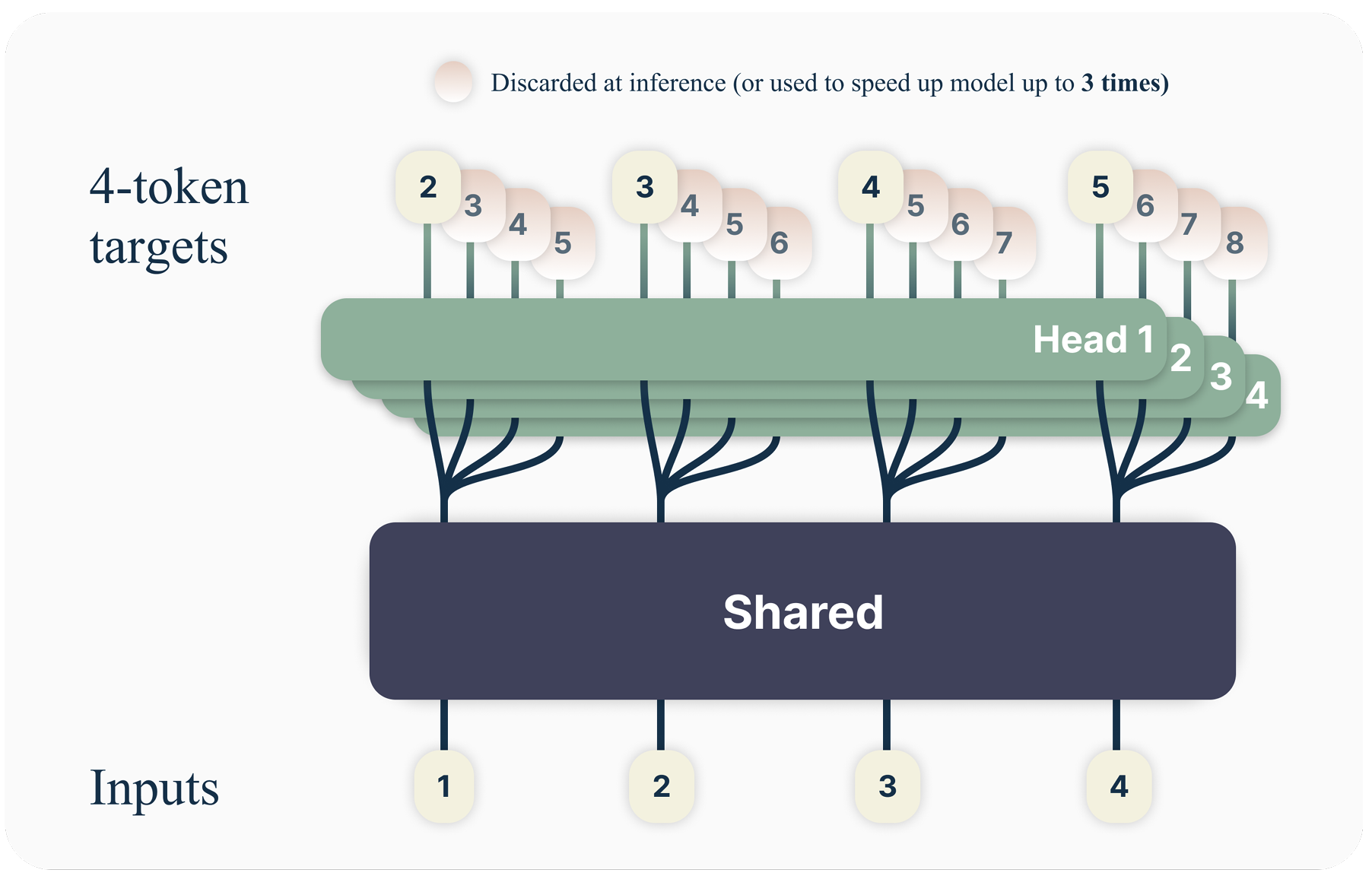
The MTP module structure of DS can be simply summarized in one sentence: DS's MTP uses \(D\) sequential modules to predict \(D\) tokens. These \(D\) modules share embedding \(\text{Emb}(\cdot)\) and output head \(\text{OutHead}(\cdot)\). The MTP module of the \(k\)th token has a dedicated transformer block \(\text{TRM}_k(\cdot)\) and a projection matrix \(M_k \in \mathbb{R}^{d \times 2d}\).

DeepSeek V3 MTP: Use D MTP module and \(k\)-th module predict \(k\)-depth token

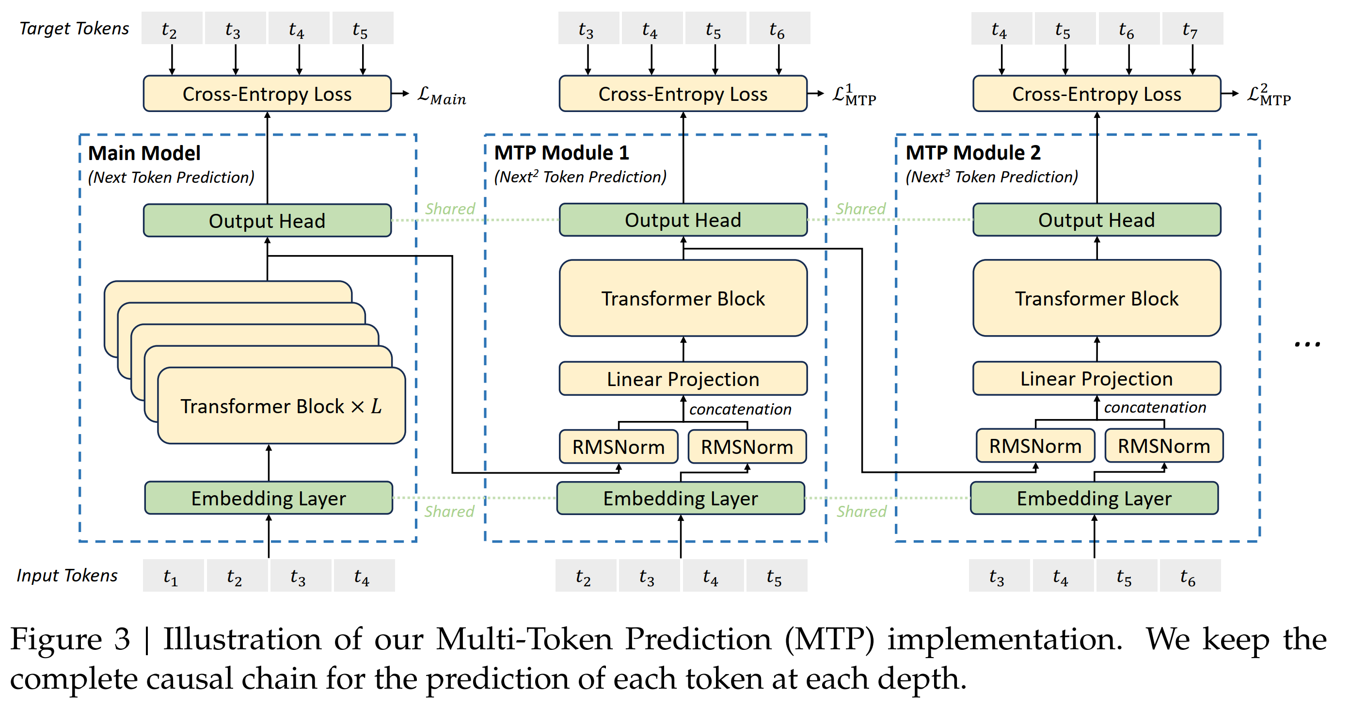
prediction：For the \(i\)th token \(t_i\) of the input sequence, at the \(k\)th prediction depth (that is, predict \(t_{i+k+1}\) below), the MTP module: 1) First get the representation \(\mathbf{h}_i^{k-1} \in \mathbb{R}^{d}\) of the \(i\)-th token at the \((k-1)\)-th depth, and the embediding \(Emb(t_{i+k}) \in \mathbb{R}^{d}\) of the \((i+k)\)-th token; 2) Then concat them (length is \(2d\)), and then generate a new representation \(h’^k_i = M_k [\text{RMSNorm}(\mathbf{h}_i^{k-1}); \text{RMSNorm}(Emb(t_{i+k}))]\) through RMSNorm and the projection matrix \(M_k \in \mathbb{R}^{d \times 2d}\); 3) Then \(\mathbf{h}’^k_i\) is taken as input to the \(k\)-th transformer module \(\text{TRM}_k(\cdot)\) to generate the output representation of the current depth \(\mathbf{h}^k_{1:T-k} = TRM_k(\mathbf{h}’^{k}_{1:T-k})\); finally, \(\text{OutHead}\) is used to convert \(\mathbf{h}^k_i\) into predicted probability \(p_{i+k+1} = OutHead(\mathbf{h}^k_i) \in \mathbb{R}^{V}\).

My understanding with the example step by step:

1. Traditional next token prediction: \(t_1\)-> \(h_1\) -> \(\hat{t}_2\), \(t_2\) -> ​​\(h_2\) -> ​​\(\hat{t}_3\), .... This is what the main model does.

2. In the \(k\)-th MTP module of DS, the model will get the \(k\)-depth representation \(\mathbf{h}_i^k\) based on the \((k-1)\)-depth MTP representation \(h_i^{k-1}\) and the embedding of token \(t_{i+k}\), and then further predict the \((k+1)\)-th token. Below, we use \(k=1, 2, 3\) as an example to illustrate how it works. Specifically, for input token \(i\):

   • When \(k=1\), first concatenate the representation \(h_i^{k-1}=h_i^0\) (from main model) of \(t_i\) and the embedding of token \(t_{i+1}\) (\(i+k=i+1\)) to get \(h’^1_i\), then input \(TRM_1\), get \(\mathbf{h}^1_{1:T-1} = TRM_1(\mathbf{h}’^{1}_{1:T-1})\), and finally get the prediction distribution \(p_{i+2}\) of token \(t_{i+2}\)

   • When \(k=2\), first concatenate the representation \(h_i^{k-1}=h_i^1\) (from \(k=1\) MTP module) of \(t_i\) and the embedding of token \(t_{i+1}\) (\(i+k=i+1\)) to get \(h’^1_i\). Then input \(TRM_1\), get \(\mathbf{h}^1_{1:T-1} = TRM_1(\mathbf{h}’^{1}_{1:T-1})\), and finally get the prediction distribution \(p_{i+2}\) of token \(t_{i+2}\). The embeddings of \(t_{i+2}\) ( \(i+k=i+2\) ) are concatenated to get \(h’^2_i\), and then input into \(TRM_2\), to get \(\mathbf{h}^2_{1:T-2} = TRM_2(\mathbf{h}’^{2}_{1:T-2})\), and finally get the prediction distribution \(p_{i+3}\) of token \(t_{i+3}\)

   • When \(k=3\), first concatenate the representation \(h_i^{k-1}=h_i^2\) (from \(k=2\) MTP module) of \(t_{i+3}\) and the embeddings of token \(t_{i+3}\) ( \(i+k=i+3\) ) to get \(h’^3_i\), and then input into \(\text{TRM}_3\), to get \(\mathbf{h}^3_{1:T-3} = TRM_3(\mathbf{h}’^{3}_{1:T-3})\), and finally get the prediction distribution \(p_{i+4}\) of token \(t_{i+4}\)

Objective function of MTP For each predicted depth k, its loss function is still cross-entropy, defined as \(\mathcal{L}_{\text{MTP}}^k\) = \(\mathcal{L}_{\text{MTP}}^k\) = \(\text{CrossEntropy}(P_{2+k:T+1}^{k}, t_{2+k:T+1})\) = \(-\frac{1}{T} \sum_{i=2+k}^{T+1} \log p_i^k[t_i]\). Where \(T\) is the length of the input sequence, \(t_i\) is the \(i\)-th true value of the input sequence, and \(p_i^k[t_i]\) is the prediciton probability of the \(k\)-th MTP module for \(t_i\).

The final MTP loss function is the average of all predicted depths (\(k\) from 1 to \(D\)) multiplied by the weight \(\lambda\), \(\mathcal{L}_{\text{MTP}}\) = \(\frac{\lambda}{D} \sum_{k=1}^{D} \mathcal{L}_{\text{MTP}}^k\)

From DS's paper formula 25, \(\mathcal{L}_{\text{MTP}}\) is only the loss function of MTP. The final loss function should also add \(\mathcal{L}_{\text{Main}}\).

How to use MTP during inference? The main purpose of MTP is to improve the performance of the main model. During inference, MTP is not used, but only the main model is used to predict the next token.

stay tuned!

Reference

1. DeepSeek-V3 Technical Report