3 - Regression with Categorical Predictors
Chapter Outline
3.0 Regression with categorical predictors
3.1 Regression with a 0/1 variable
3.2 Regression with a 1/2 variable
3.3 Regression with a 1/2/3 variable
3.4 Regression with multiple categorical predictors
3.5 Categorical predictor with interactions
3.6 Continuous and categorical variables
3.7 Interactions of continuous by 0/1 categorical variables
3.8 Continuous and categorical variables, interaction with 1/2/3 variable
3.9 Summary
3.10 For more information
3.0 Introduction
In the previous two chapters, we have focused on regression analyses using continuous variables. However, it is possible to include categorical predictors in a regression analysis, but it requires some extra work in performing the analysis and extra work in properly interpreting the results. This chapter will illustrate how you can use Python for including categorical predictors in your analysis and describe how to interpret the results of such analyses.
This chapter will use the elemapi2 data that you have seen in the prior chapters. We will focus on four variables api00, some_col, yr_rnd and mealcat, which takes meals and breaks it up into three categories. Let's have a quick look at these variables.
import pandas as pd
import numpy as np
import itertools
from itertools import chain, combinations
import statsmodels.formula.api as smf
import scipy.stats as scipystats
import statsmodels.api as sm
import statsmodels.stats.stattools as stools
import statsmodels.stats as stats
from statsmodels.graphics.regressionplots import *
import matplotlib.pyplot as plt
import seaborn as sns
import copy
from sklearn.cross_validation import train_test_split
import math
import time

%matplotlib inline
plt.rcParams['figure.figsize'] = (8, 6)

mypath =  r'F:\Dropbox\ipynb_notes\ipynb_blog\\'

elemapi2 = pd.read_csv(mypath + r'elemapi2.csv')
elemapi2_sel = elemapi2.ix[:, ["api00", "some_col", "yr_rnd", "mealcat"]]
print elemapi2_sel.describe()

def cv_desc(df, var):
    return df[var].value_counts(dropna = False)

print '\n'
print cv_desc(elemapi2_sel, 'mealcat')
print '\n'
print cv_desc(elemapi2_sel, 'yr_rnd')
            api00    some_col     yr_rnd     mealcat
count  400.000000  400.000000  400.00000  400.000000
mean   647.622500   19.712500    0.23000    2.015000
std    142.248961   11.336938    0.42136    0.819423
min    369.000000    0.000000    0.00000    1.000000
25%    523.750000   12.000000    0.00000    1.000000
50%    643.000000   19.000000    0.00000    2.000000
75%    762.250000   28.000000    0.00000    3.000000
max    940.000000   67.000000    1.00000    3.000000


3    137
2    132
1    131
Name: mealcat, dtype: int64


0    308
1     92
Name: yr_rnd, dtype: int64
The variable api00 is a measure of the performance of the students. The variable some_col is a continuous variable that measures the percentage of the parents in the school who have attended college. The variable yr_rnd is a categorical variable that is coded 0 if the school is not year round, and 1 if year round. The variable meals is the percentage of students who are receiving state sponsored free meals and can be used as an indicator of poverty. This was broken into 3 categories (to make equally sized groups) creating the variable mealcat. The following macro function created for this dataset gives us codebook type information on a variable that we specify. It gives the information of the number of unique values that a variable take.
def codebook(df, var):
    title = "Codebook for " + str(var)
    unique_values = len(df[var].unique())
    max_v = df[var].max()
    min_v = df[var].min()
    n_miss = sum(pd.isnull(df[var]))
    mean = df[var].mean()
    stdev = df[var].std()
    print pd.DataFrame({'title': title, 'unique values': unique_values, 'max value' : max_v, 'min value': min_v, 'num of missing' : n_miss, 'mean' : mean, 'stdev' : stdev}, index = [0])
    return

codebook(elemapi2_sel, 'api00')
   max value      mean  min value  num of missing       stdev  \
0        940  647.6225        369               0  142.248961

                title  unique values
0  Codebook for api00            271
3.1 Regression with a 0/1 variable
The simplest example of a categorical predictor in a regression analysis is a 0/1 variable, also called a dummy variable or sometimes an indicator variable. Let's use the variable yr_rnd as an example of a dummy variable. We can include a dummy variable as a predictor in a regression analysis as shown below.
reg = smf.ols(formula = "api00 ~ yr_rnd", data = elemapi2_sel).fit()
reg.summary()
| Dep. Variable: | api00 | R-squared: | 0.226 |
|---|---|---|---|
| Model: | OLS | Adj. R-squared: | 0.224 |
| Method: | Least Squares | F-statistic: | 116.2 |
| Date: | Sun, 22 Jan 2017 | Prob (F-statistic): | 5.96e-24 |
| Time: | 14:04:29 | Log-Likelihood: | -2498.9 |
| No. Observations: | 400 | AIC: | 5002. |
| Df Residuals: | 398 | BIC: | 5010. |
| Df Model: | 1 | ||
| Covariance Type: | nonrobust |
| coef | std err | t | P>|t| | [95.0% Conf. Int.] | |
|---|---|---|---|---|---|
| Intercept | 684.5390 | 7.140 | 95.878 | 0.000 | 670.503 698.575 |
| yr_rnd | -160.5064 | 14.887 | -10.782 | 0.000 | -189.774 -131.239 |
| Omnibus: | 45.748 | Durbin-Watson: | 1.499 |
|---|---|---|---|
| Prob(Omnibus): | 0.000 | Jarque-Bera (JB): | 13.162 |
| Skew: | 0.006 | Prob(JB): | 0.00139 |
| Kurtosis: | 2.111 | Cond. No. | 2.53 |
This may seem odd at first, but this is a legitimate analysis. But what does this mean? Let's go back to basics and write out the regression equation that this model implies.
api00 = Intercept + Byr_rnd * yr_rnd
where Intercept is the intercept (or constant) and we use Byr_rnd to represent the coefficient for variable yr_rnd. Filling in the values from the regression equation, we get
api00 = 684.539 + -160.5064 * yr_rnd
If a school is not a year-round school (i.e., yr_rnd is 0) the regression equation would simplify to
api00 = constant    + 0 * Byr_rnd
api00 = 684.539     + 0 * -160.5064
api00 = 684.539
If a school is a year-round school, the regression equation would simplify to
api00 = constant + 1 * Byr_rnd
api00 = 684.539  + 1 * -160.5064
api00 = 524.0326
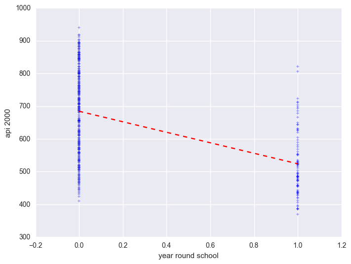
We can graph the observed values and the predicted values as shown below. Although yr_rnd only has two values, we can still draw a regression line showing the relationship between yr_rnd and api00. Based on the results above, we see that the predicted value for non-year round schools is 684.539 and the predicted value for the year round schools is 524.032, and the slope of the line is negative, which makes sense since the coefficient for yr_rnd was negative (-160.5064).
plt.scatter(elemapi2_sel.yr_rnd, elemapi2_sel.api00, marker = "+")
plt.plot([0, 1], [np.mean(elemapi2_sel.query('yr_rnd == 0').api00), np.mean(elemapi2_sel.query('yr_rnd == 1').api00)], 'r--')
plt.ylabel("api 2000")
plt.xlabel("year round school")
plt.show()
Let's compare these predicted values to the mean api00 scores for the year-round and non-year-round students. Let's create a format for variable yr_rnd and mealcat so we can label these categorical variables. Notice that we use the format statement in groupby aggregate mean below to show value labels for variable yr_rnd.
elemapi2_sel["yr_rnd_c"] = elemapi2_sel.yr_rnd.map({0: "No", 1: "Yes"})
elemapi2_sel["mealcat_c"] = elemapi2_sel.mealcat.map({1: "0-46% free meals", 2: "47-80% free meals", 3: "1-100% free meals"})

elemapi2_sel_group = elemapi2_sel.groupby("yr_rnd_c")
elemapi2_sel_group.api00.agg([np.mean, np.std])
| mean | std | |
|---|---|---|
| yr_rnd_c | ||
| No | 684.538961 | 132.112534 |
| Yes | 524.032609 | 98.916043 |
As you see, the regression equation predicts that for a school, the value of api00 will be the mean value of the group determined by the school type.
Let's relate these predicted values back to the regression equation. For the non-year-round schools, their mean is the same as the intercept (684.539). The coefficient for yr_rnd is the amount we need to add to get the mean for the year-round schools, i.e., we need to add -160.5064 to get 524.0326, the mean for the non year-round schools. In other words, Byr_rnd is the mean api00 score for the year-round schools minus the mean api00 score for the non year-round schools, i.e., mean(year-round) - mean(non year-round).
It may be surprising to note that this regression analysis with a single dummy variable is the same as doing a t-test comparing the mean api00 for the year-round schools with the non year-round schools (see below). You can see that the t value below is the same as the t value for yr_rnd in the regression above. This is because Byr_rnd compares the non year-rounds and non year-rounds (since the coefficient is mean(year round)-mean(non year-round)).
# pooled ttest, assume equal population variance
print scipystats.ttest_ind(elemapi2_sel.query('yr_rnd == 0').api00, elemapi2_sel.query('yr_rnd == 1').api00)

# does not assume equal variance
print scipystats.ttest_ind(elemapi2_sel.query('yr_rnd == 0').api00, elemapi2_sel.query('yr_rnd == 1').api00, equal_var = False)
Ttest_indResult(statistic=10.781500136400451, pvalue=5.9647081127888056e-24)
Ttest_indResult(statistic=12.57105956566846, pvalue=5.2973148066493157e-27)
Since a t-test is the same as doing an anova, we can get the same results using anova as well.
print scipystats.f_oneway(elemapi2_sel.query('yr_rnd == 0').api00, elemapi2_sel.query('yr_rnd == 1').api00)
F_onewayResult(statistic=116.2407451912029, pvalue=5.9647081127907988e-24)
If we square the t-value from the t-test, we get the same value as the F-value from anova: 10.78^2=116.21 (with a little rounding error.)
3.2 Regression with a 1/2 variable
A categorical predictor variable does not have to be coded 0/1 to be used in a regression model. It is easier to understand and interpret the results from a model with dummy variables, but the results from a variable coded 1/2 yield essentially the same results.
Lets make a copy of the variable yr_rnd called yr_rnd2 that is coded 1/2, 1=non year-round and 2=year-round.
elemapi2_sel["yr_rnd2"] = elemapi2_sel["yr_rnd"] + 1
reg = smf.ols("api00 ~ yr_rnd2", data = elemapi2_sel).fit()
reg.summary()
| Dep. Variable: | api00 | R-squared: | 0.226 |
|---|---|---|---|
| Model: | OLS | Adj. R-squared: | 0.224 |
| Method: | Least Squares | F-statistic: | 116.2 |
| Date: | Sun, 22 Jan 2017 | Prob (F-statistic): | 5.96e-24 |
| Time: | 14:15:36 | Log-Likelihood: | -2498.9 |
| No. Observations: | 400 | AIC: | 5002. |
| Df Residuals: | 398 | BIC: | 5010. |
| Df Model: | 1 | ||
| Covariance Type: | nonrobust |
| coef | std err | t | P>|t| | [95.0% Conf. Int.] | |
|---|---|---|---|---|---|
| Intercept | 845.0453 | 19.353 | 43.664 | 0.000 | 806.998 883.093 |
| yr_rnd2 | -160.5064 | 14.887 | -10.782 | 0.000 | -189.774 -131.239 |
| Omnibus: | 45.748 | Durbin-Watson: | 1.499 |
|---|---|---|---|
| Prob(Omnibus): | 0.000 | Jarque-Bera (JB): | 13.162 |
| Skew: | 0.006 | Prob(JB): | 0.00139 |
| Kurtosis: | 2.111 | Cond. No. | 6.23 |
Note that the coefficient for yr_rnd is the same as yr_rnd2. So, you can see that if you code yr_rnd as 0/1 or as 1/2, the regression coefficient works out to be the same. However the intercept (Intercept) is a bit less intuitive. When we used yr_rnd, the intercept was the mean for the non year-rounds. When using yr_rnd2, the intercept is the mean for the non year-rounds minus Byr_rnd2, i.e., 684.539 - (-160.506) = 845.045
Note that you can use 0/1 or 1/2 coding and the results for the coefficient come out the same, but the interpretation of constant in the regression equation is different. It is often easier to interpret the estimates for 0/1 coding.
In summary, these results indicate that the api00 scores are significantly different for the schools depending on the type of school, year round school versus non-year round school. Non year-round schools have significantly higher API scores than year-round schools. Based on the regression results, non year-round schools have scores that are 160.5 points higher than year-round schools.
3.3 Regression with a 1/2/3 variable
3.3.1 Manually creating dummy variables
Say, that we would like to examine the relationship between the amount of poverty and api scores. We don't have a measure of poverty, but we can use mealcat as a proxy for a measure of poverty. From the previous section, we have seen that variable mealcat has three unique values. These are the levels of percent of students on free meals. We can associate a value label to variable mealcat to make it more meaningful for us when we run python regression with mealcat.
elemapi2_sel_group = elemapi2_sel.groupby("mealcat_c")
elemapi2_sel_group.api00.agg([lambda x: x.shape[0], np.mean, np.std])
| <lambda> | mean | std | |
|---|---|---|---|
| mealcat_c | |||
| 0-46% free meals | 131 | 805.717557 | 65.668664 |
| 1-100% free meals | 137 | 504.379562 | 62.727015 |
| 47-80% free meals | 132 | 639.393939 | 82.135130 |
lm = smf.ols('api00 ~ mealcat', data = elemapi2_sel).fit()
lm.summary()
| Dep. Variable: | api00 | R-squared: | 0.752 |
|---|---|---|---|
| Model: | OLS | Adj. R-squared: | 0.752 |
| Method: | Least Squares | F-statistic: | 1208. |
| Date: | Sun, 22 Jan 2017 | Prob (F-statistic): | 1.29e-122 |
| Time: | 14:17:37 | Log-Likelihood: | -2271.1 |
| No. Observations: | 400 | AIC: | 4546. |
| Df Residuals: | 398 | BIC: | 4554. |
| Df Model: | 1 | ||
| Covariance Type: | nonrobust |
| coef | std err | t | P>|t| | [95.0% Conf. Int.] | |
|---|---|---|---|---|---|
| Intercept | 950.9874 | 9.422 | 100.935 | 0.000 | 932.465 969.510 |
| mealcat | -150.5533 | 4.332 | -34.753 | 0.000 | -159.070 -142.037 |
| Omnibus: | 3.106 | Durbin-Watson: | 1.516 |
|---|---|---|---|
| Prob(Omnibus): | 0.212 | Jarque-Bera (JB): | 3.112 |
| Skew: | -0.214 | Prob(JB): | 0.211 |
| Kurtosis: | 2.943 | Cond. No. | 6.86 |
This is looking at the linear effect of mealcat with api00, but mealcat is not an interval variable. Instead, you will want to code the variable so that all the information concerning the three levels is accounted for. In general, we need to go through a data step to create dummy variables. For example, in order to create dummy variables for mealcat, we can do the following using sklearn to create dummy variables.
from sklearn import preprocessing
le_mealcat = preprocessing.LabelEncoder()
elemapi2_sel['mealcat_dummy'] = le_mealcat.fit_transform(elemapi2_sel.mealcat)

elemapi2_sel.groupby('mealcat_dummy').size()


ohe = preprocessing.OneHotEncoder()
dummy = pd.DataFrame(ohe.fit_transform(elemapi2_sel.mealcat.reshape(-1,1)).toarray(), columns = ["mealcat1", "mealcat2", "mealcat3"])
elemapi2_sel = pd.concat([elemapi2_sel, dummy], axis = 1)
lm = smf.ols('api00 ~ mealcat2 + mealcat3', data = elemapi2_sel).fit()
lm.summary()
| Dep. Variable: | api00 | R-squared: | 0.755 |
|---|---|---|---|
| Model: | OLS | Adj. R-squared: | 0.754 |
| Method: | Least Squares | F-statistic: | 611.1 |
| Date: | Sun, 22 Jan 2017 | Prob (F-statistic): | 6.48e-122 |
| Time: | 14:20:30 | Log-Likelihood: | -2269.0 |
| No. Observations: | 400 | AIC: | 4544. |
| Df Residuals: | 397 | BIC: | 4556. |
| Df Model: | 2 | ||
| Covariance Type: | nonrobust |
| coef | std err | t | P>|t| | [95.0% Conf. Int.] | |
|---|---|---|---|---|---|
| Intercept | 805.7176 | 6.169 | 130.599 | 0.000 | 793.589 817.846 |
| mealcat2[0] | -83.1618 | 4.354 | -19.099 | 0.000 | -91.722 -74.602 |
| mealcat2[1] | -83.1618 | 4.354 | -19.099 | 0.000 | -91.722 -74.602 |
| mealcat3[0] | -150.6690 | 4.314 | -34.922 | 0.000 | -159.151 -142.187 |
| mealcat3[1] | -150.6690 | 4.314 | -34.922 | 0.000 | -159.151 -142.187 |
| Omnibus: | 1.593 | Durbin-Watson: | 1.541 |
|---|---|---|---|
| Prob(Omnibus): | 0.451 | Jarque-Bera (JB): | 1.684 |
| Skew: | -0.139 | Prob(JB): | 0.431 |
| Kurtosis: | 2.847 | Cond. No. | 2.14e+16 |
The interpretation of the coefficients is much like that for the binary variables. Group 1 is the omitted group, so Intercept is the mean for group 1. The coefficient for mealcat2 is the mean for group 2 minus the mean of the omitted group (group 1). And the coefficient for mealcat3 is the mean of group 3 minus the mean of group 1. You can verify this by comparing the coefficients with the means of the groups.
elemapi2_sel.groupby("mealcat").api00.mean()
mealcat
1    805.717557
2    639.393939
3    504.379562
Name: api00, dtype: float64
Based on these results, we can say that the three groups differ in their api00 scores, and that in particular group 2 is significantly different from group1 (because mealcat2 was significant) and group 3 is significantly different from group 1 (because mealcat3 was significant).
3.3.2 More on dummy coding
Of course, there is the way of coding by hand. I will ignore it here.
3.3.3 run regression with categorical variable directly
lm = lm = smf.ols('api00 ~ C(mealcat)', data = elemapi2_sel).fit()
lm.summary()
| Dep. Variable: | api00 | R-squared: | 0.755 |
|---|---|---|---|
| Model: | OLS | Adj. R-squared: | 0.754 |
| Method: | Least Squares | F-statistic: | 611.1 |
| Date: | Sun, 22 Jan 2017 | Prob (F-statistic): | 6.48e-122 |
| Time: | 14:21:59 | Log-Likelihood: | -2269.0 |
| No. Observations: | 400 | AIC: | 4544. |
| Df Residuals: | 397 | BIC: | 4556. |
| Df Model: | 2 | ||
| Covariance Type: | nonrobust |
| coef | std err | t | P>|t| | [95.0% Conf. Int.] | |
|---|---|---|---|---|---|
| Intercept | 805.7176 | 6.169 | 130.599 | 0.000 | 793.589 817.846 |
| C(mealcat)[T.2] | -166.3236 | 8.708 | -19.099 | 0.000 | -183.444 -149.203 |
| C(mealcat)[T.3] | -301.3380 | 8.629 | -34.922 | 0.000 | -318.302 -284.374 |
| Omnibus: | 1.593 | Durbin-Watson: | 1.541 |
|---|---|---|---|
| Prob(Omnibus): | 0.451 | Jarque-Bera (JB): | 1.684 |
| Skew: | -0.139 | Prob(JB): | 0.431 |
| Kurtosis: | 2.847 | Cond. No. | 3.76 |
3.3.4 Other coding schemes
It is generally very convenient to use dummy coding but it is not the only kind of coding that can be used. As you have seen, when you use dummy coding one of the groups becomes the reference group and all of the other groups are compared to that group. This may not be the most interesting set of comparisons.
Say you want to compare group 1 with 2, and group 2 with group 3. You need to generate a coding scheme that forms these 2 comparisons. In python, we can first generate the corresponding coding scheme in a data step shown below and use them in the regression.
We create two dummy variables, one for group 1 and the other for group 3.
elemapi2_sel = elemapi2.ix[:, ["api00", "some_col", "yr_rnd", "mealcat"]]

elemapi2_sel["mealcat1"] = np.where(elemapi2_sel.mealcat == 1, 2.0 / 3, -1.0/3)
elemapi2_sel["mealcat2"] = np.where(elemapi2_sel.mealcat == 2, 2.0 / 3, -1.0/3)
elemapi2_sel["mealcat3"] = np.where(elemapi2_sel.mealcat == 3, 2.0 / 3, -1.0/3)

elemapi2_sel.groupby(["mealcat", "mealcat1",  "mealcat3"]).size()
mealcat  mealcat1   mealcat3
1         0.666667  -0.333333    131
2        -0.333333  -0.333333    132
3        -0.333333   0.666667    137
dtype: int64
lm = lm = smf.ols('api00 ~ mealcat1 + mealcat3', data = elemapi2_sel).fit()
lm.summary()
| Dep. Variable: | api00 | R-squared: | 0.755 |
|---|---|---|---|
| Model: | OLS | Adj. R-squared: | 0.754 |
| Method: | Least Squares | F-statistic: | 611.1 |
| Date: | Mon, 09 Jan 2017 | Prob (F-statistic): | 6.48e-122 |
| Time: | 00:19:01 | Log-Likelihood: | -2269.0 |
| No. Observations: | 400 | AIC: | 4544. |
| Df Residuals: | 397 | BIC: | 4556. |
| Df Model: | 2 | ||
| Covariance Type: | nonrobust |
| coef | std err | t | P>|t| | [95.0% Conf. Int.] | |
|---|---|---|---|---|---|
| Intercept | 649.8304 | 3.531 | 184.021 | 0.000 | 642.888 656.773 |
| mealcat1 | 166.3236 | 8.708 | 19.099 | 0.000 | 149.203 183.444 |
| mealcat3 | -135.0144 | 8.612 | -15.677 | 0.000 | -151.945 -118.083 |
| Omnibus: | 1.593 | Durbin-Watson: | 1.541 |
|---|---|---|---|
| Prob(Omnibus): | 0.451 | Jarque-Bera (JB): | 1.684 |
| Skew: | -0.139 | Prob(JB): | 0.431 |
| Kurtosis: | 2.847 | Cond. No. | 3.01 |
If you compare the parameter estimates with the group means of mealcat you can verify that B1 (i.e. 0-46% free meals) is the mean of group 1 minus group 2, and B2 (i.e., 47-80% free meals) is the mean of group 2 minus group 3. Both of these comparisons are significant, indicating that group 1 significantly differs from group 2, and group 2 significantly differs from group 3.
And the value of the intercept term Intercept is the unweighted average of the means of the three groups, (805.71756 +639.39394 +504.37956)/3 = 649.83035.
3.4 Regression with two categorical predictors
3.4.1 Manually creating dummy variables
Previously we looked at using yr_rnd to predict api00 and we have also looked at using mealcat to predict api00. Let's include the parameter estimates for each model below.
lm = smf.ols('api00 ~ yr_rnd', data = elemapi2_sel).fit()
print lm.summary()

print '\n'

lm = smf.ols('api00 ~ mealcat1 + mealcat2', data = elemapi2_sel).fit()
print lm.summary()
                            OLS Regression Results
==============================================================================
Dep. Variable:                  api00   R-squared:                       0.226
Model:                            OLS   Adj. R-squared:                  0.224
Method:                 Least Squares   F-statistic:                     116.2
Date:                Sun, 22 Jan 2017   Prob (F-statistic):           5.96e-24
Time:                        14:23:42   Log-Likelihood:                -2498.9
No. Observations:                 400   AIC:                             5002.
Df Residuals:                     398   BIC:                             5010.
Df Model:                           1
Covariance Type:            nonrobust
==============================================================================
                 coef    std err          t      P>|t|      [95.0% Conf. Int.]
------------------------------------------------------------------------------
Intercept    684.5390      7.140     95.878      0.000       670.503   698.575
yr_rnd      -160.5064     14.887    -10.782      0.000      -189.774  -131.239
==============================================================================
Omnibus:                       45.748   Durbin-Watson:                   1.499
Prob(Omnibus):                  0.000   Jarque-Bera (JB):               13.162
Skew:                           0.006   Prob(JB):                      0.00139
Kurtosis:                       2.111   Cond. No.                         2.53
==============================================================================

Warnings:
[1] Standard Errors assume that the covariance matrix of the errors is correctly specified.


                            OLS Regression Results
==============================================================================
Dep. Variable:                  api00   R-squared:                       0.755
Model:                            OLS   Adj. R-squared:                  0.754
Method:                 Least Squares   F-statistic:                     611.1
Date:                Sun, 22 Jan 2017   Prob (F-statistic):          6.48e-122
Time:                        14:23:42   Log-Likelihood:                -2269.0
No. Observations:                 400   AIC:                             4544.
Df Residuals:                     397   BIC:                             4556.
Df Model:                           2
Covariance Type:            nonrobust
==============================================================================
                 coef    std err          t      P>|t|      [95.0% Conf. Int.]
------------------------------------------------------------------------------
Intercept    649.8304      3.531    184.021      0.000       642.888   656.773
mealcat1     301.3380      8.629     34.922      0.000       284.374   318.302
mealcat2     135.0144      8.612     15.677      0.000       118.083   151.945
==============================================================================
Omnibus:                        1.593   Durbin-Watson:                   1.541
Prob(Omnibus):                  0.451   Jarque-Bera (JB):                1.684
Skew:                          -0.139   Prob(JB):                        0.431
Kurtosis:                       2.847   Cond. No.                         2.98
==============================================================================

Warnings:
[1] Standard Errors assume that the covariance matrix of the errors is correctly specified.
In the first model with only yr_rnd as the only predictor, the intercept term is the mean api score for the non-year-round schools. The coefficient for yr_rnd is the difference between the year round and non-year round group. In the second model, the coefficient for mealcat1 is the difference between mealcat=1 and mealcat=3, and the coefficient for mealcat2 is the difference between mealcat=2 and mealcat=3. The intercept is the mean for the mealcat=3.
Of course, we can include both yr_rnd and mealcat together in the same model. Now the question is how to interpret the coefficients.
lm = smf.ols('api00 ~ yr_rnd + mealcat1 + mealcat2', data = elemapi2_sel).fit()
print lm.summary()
                            OLS Regression Results
==============================================================================
Dep. Variable:                  api00   R-squared:                       0.767
Model:                            OLS   Adj. R-squared:                  0.765
Method:                 Least Squares   F-statistic:                     435.0
Date:                Mon, 09 Jan 2017   Prob (F-statistic):          6.40e-125
Time:                        21:18:55   Log-Likelihood:                -2258.6
No. Observations:                 400   AIC:                             4525.
Df Residuals:                     396   BIC:                             4541.
Df Model:                           3
Covariance Type:            nonrobust
==============================================================================
                 coef    std err          t      P>|t|      [95.0% Conf. Int.]
------------------------------------------------------------------------------
Intercept    659.5396      4.043    163.126      0.000       651.591   667.488
yr_rnd       -42.9601      9.362     -4.589      0.000       -61.365   -24.555
mealcat1     281.6832      9.446     29.821      0.000       263.113   300.253
mealcat2     117.9458      9.189     12.836      0.000        99.881   136.011
==============================================================================
Omnibus:                        1.210   Durbin-Watson:                   1.584
Prob(Omnibus):                  0.546   Jarque-Bera (JB):                1.279
Skew:                          -0.086   Prob(JB):                        0.528
Kurtosis:                       2.783   Cond. No.                         3.95
==============================================================================

Warnings:
[1] Standard Errors assume that the covariance matrix of the errors is correctly specified.
Let's dig below the surface and see how the coefficients relate to the predicted values. Let's view the cells formed by crossing yr_rnd and mealcat and number the cells from cell1 to cell6.
| | mealcat=1 | mealcat=2 | mealcat=3 |
|--: |--: |--: |--: |--: |
| yr_rnd=0 | cell1 | cell2 | cell3 |
| yr_rnd=1 | cell4 | cell5 | cell6 |
With respect to mealcat, the group mealcat=3 is the reference category, and with respect to yr_rnd the group yr_rnd=0 is the reference category. As a result, cell3 is the reference cell. The intercept is the predicted value for this cell.
The coefficient for yr_rnd is the difference between cell3 and cell6. Since this model has only main effects, it is also the difference between cell2 and cell5, or from cell1 and cell4. In other words, Byr_rnd is the amount you add to the predicted value when you go from non-year round to year round schools.
The coefficient for mealcat1 is the predicted difference between cell1 and cell3. Since this model only has main effects, it is also the predicted difference between cell4 and cell6. Likewise, Bmealcat2 is the predicted difference between cell2 and cell3, and also the predicted difference between cell5 and cell6.
So, the predicted values, in terms of the coefficients, would be
| | mealcat=1 | mealcat=2 | mealcat=3 |
|--: |--: |--: |--: |--: |
| yr_rnd=0 | Intercept + Bmealcat1 | Intercept + Bmealcat2 | Intercept |
| yr_rnd=1 | Intercept + Byr_rnd + Bmealcat1 | Intercept + Byr_rnd + Bmealcat2 | Intercept + Byr_rnd |
We should note that if you computed the predicted values for each cell, they would not exactly match the means in the six cells. The predicted means would be close to the observed means in the cells, but not exactly the same. This is because our model only has main effects and assumes that the difference between cell1 and cell4 is exactly the same as the difference between cells 2 and 5 which is the same as the difference between cells 3 and 5. Since the observed values don't follow this pattern, there is some discrepancy between the predicted means and observed means.
3.4.2 Using the C formula directly
We can run the same analysis using the categorical formula without manually coding the dummy variables.
lm = smf.ols('api00 ~ yr_rnd + C(mealcat)', data = elemapi2_sel).fit()
print lm.summary()
                            OLS Regression Results
==============================================================================
Dep. Variable:                  api00   R-squared:                       0.767
Model:                            OLS   Adj. R-squared:                  0.765
Method:                 Least Squares   F-statistic:                     435.0
Date:                Sun, 22 Jan 2017   Prob (F-statistic):          6.40e-125
Time:                        14:24:47   Log-Likelihood:                -2258.6
No. Observations:                 400   AIC:                             4525.
Df Residuals:                     396   BIC:                             4541.
Df Model:                           3
Covariance Type:            nonrobust
===================================================================================
                      coef    std err          t      P>|t|      [95.0% Conf. Int.]
-----------------------------------------------------------------------------------
Intercept         808.0131      6.040    133.777      0.000       796.139   819.888
C(mealcat)[T.2]  -163.7374      8.515    -19.229      0.000      -180.478  -146.997
C(mealcat)[T.3]  -281.6832      9.446    -29.821      0.000      -300.253  -263.113
yr_rnd            -42.9601      9.362     -4.589      0.000       -61.365   -24.555
==============================================================================
Omnibus:                        1.210   Durbin-Watson:                   1.584
Prob(Omnibus):                  0.546   Jarque-Bera (JB):                1.279
Skew:                          -0.086   Prob(JB):                        0.528
Kurtosis:                       2.783   Cond. No.                         4.17
==============================================================================

Warnings:
[1] Standard Errors assume that the covariance matrix of the errors is correctly specified.
In summary, these results indicate the differences between year round and non-year round schools is significant, and the differences among the three mealcat groups are significant.
3.5 Categorical predictor with interactions
3.5.1 Manually creating dummy variables
Let's perform the same analysis that we performed above, this time let's include the interaction of mealcat by yr_rnd. In this section we show how to do it by manually creating all the dummy variables. We use the array structure again. This time we have to declare two set of arrays, one for the dummy variables of mealcat and one for the interaction of yr_rnd and mealcat.
elemapi2_sel = elemapi2.ix[:, ["api00", "some_col", "yr_rnd", "mealcat"]]

ohe = preprocessing.OneHotEncoder()
dummy = pd.DataFrame(ohe.fit_transform(elemapi2_sel.mealcat.reshape(-1,1)).toarray(), columns = ["mealcat1", "mealcat2", "mealcat3"])
mealxynd = np.multiply(dummy, elemapi2.yr_rnd.reshape(-1, 1))
mealxynd.columns = ["mealxynd1", "mealxynd2", "mealxynd3"]
elemapi2_sel = pd.concat([elemapi2_sel, dummy, mealxynd], axis = 1)

elemapi2_sel.groupby(["yr_rnd", "mealcat", "mealxynd1", "mealxynd2", "mealxynd3"]).size()
yr_rnd  mealcat  mealxynd1  mealxynd2  mealxynd3
0       1        0.0        0.0        0.0          124
        2        0.0        0.0        0.0          117
        3        0.0        0.0        0.0           67
1       1        1.0        0.0        0.0            7
        2        0.0        1.0        0.0           15
        3        0.0        0.0        1.0           70
dtype: int64
Now let's add these dummy variables for interaction between yr_rnd and mealcat to our model. We can all add a test statement to test the overall interaction. The output shows that the interaction effect is not significant.
lm = smf.ols('api00 ~ yr_rnd + mealcat1 + mealcat2 + mealxynd1 + mealxynd2', data = elemapi2_sel).fit()
print lm.summary()
                            OLS Regression Results
==============================================================================
Dep. Variable:                  api00   R-squared:                       0.769
Model:                            OLS   Adj. R-squared:                  0.766
Method:                 Least Squares   F-statistic:                     261.6
Date:                Sun, 22 Jan 2017   Prob (F-statistic):          9.19e-123
Time:                        14:26:06   Log-Likelihood:                -2257.5
No. Observations:                 400   AIC:                             4527.
Df Residuals:                     394   BIC:                             4551.
Df Model:                           5
Covariance Type:            nonrobust
==============================================================================
                 coef    std err          t      P>|t|      [95.0% Conf. Int.]
------------------------------------------------------------------------------
Intercept    521.4925      8.414     61.978      0.000       504.950   538.035
yr_rnd       -33.4925     11.771     -2.845      0.005       -56.635   -10.350
mealcat1     288.1929     10.443     27.597      0.000       267.662   308.724
mealcat2     123.7810     10.552     11.731      0.000       103.036   144.526
mealxynd1    -40.7644     29.231     -1.395      0.164       -98.233    16.704
mealxynd2    -18.2476     22.256     -0.820      0.413       -62.003    25.508
==============================================================================
Omnibus:                        1.439   Durbin-Watson:                   1.583
Prob(Omnibus):                  0.487   Jarque-Bera (JB):                1.484
Skew:                          -0.096   Prob(JB):                        0.476
Kurtosis:                       2.771   Cond. No.                         10.4
==============================================================================

Warnings:
[1] Standard Errors assume that the covariance matrix of the errors is correctly specified.
It is important to note how the meaning of the coefficients change in the presence of these interaction terms. For example, in the prior model, with only main effects, we could interpret Byr_rnd as the difference between the year round and non year round schools. However, now that we have added the interaction term, the term Byr_rnd represents the difference between cell3 and cell6, or the difference between the year round and non-year round schools when mealcat=3 (because mealcat=3 was the omitted group). The presence of an interaction would imply that the difference between year round and non-year round schools depends on the level of mealcat. The interaction terms Bmealxynd1 and Bmealxynd2 represent the extent to which the difference between the year round/non year round schools changes when mealcat=1 and when mealcat=2 (as compared to the reference group, mealcat=3). For example the term Bmealxynd1 represents the difference between year round and non-year round for mealcat=1 versus the difference for mealcat=3. In other words, Bmealxynd1 in this design is (cell1-cell4) - (cell3-cell6), or it represents how much the effect of yr_rnd differs between mealcat=1 and mealcat=3.
Below we have shown the predicted values for the six cells in terms of the coefficients in the model. If you compare this to the main effects model, you will see that the predicted values are the same except for the addition of mealxynd1 (in cell 4) and mealxynd2 (in cell 5).
| | mealcat=1 | mealcat=2 | mealcat=3 |
|--: |--: |--: |--: |--: |
| yr_rnd=0 | Intercept + Bmealcat1 | Intercept + Bmealcat2 | Intercept |
| yr_rnd=1 | Intercept + Byr_rnd + Bmealcat1 + Bmealxynd1 | Intercept + Byr_rnd + Bmealcat2 + Bmealxynd2 | Intercept + Byr_rnd |
It can be very tricky to interpret these interaction terms if you wish to form specific comparisons. For example, if you wanted to perform a test of the simple main effect of yr_rnd when mealcat=1, i.e., comparing compare cell1 with cell4, you would want to compare Intercept+ mealcat1 versus Intercept + mealcat1 + yr_rnd + mealxynd1 and since Intercept and Imealcat1 would drop out.
3.5.2 Using anova
Constructing these interactions can be easier. We can also avoid manually coding our dummy variables. As you see below, the C formula gives us the test of the overall main effects and interactions without the need to perform subsequent test commands.
lm = smf.ols('api00 ~ C(yr_rnd) * C(mealcat)', data = elemapi2_sel).fit()
print lm.summary()
                            OLS Regression Results
==============================================================================
Dep. Variable:                  api00   R-squared:                       0.769
Model:                            OLS   Adj. R-squared:                  0.766
Method:                 Least Squares   F-statistic:                     261.6
Date:                Mon, 09 Jan 2017   Prob (F-statistic):          9.19e-123
Time:                        21:54:22   Log-Likelihood:                -2257.5
No. Observations:                 400   AIC:                             4527.
Df Residuals:                     394   BIC:                             4551.
Df Model:                           5
Covariance Type:            nonrobust
==================================================================================================
                                     coef    std err          t      P>|t|      [95.0% Conf. Int.]
--------------------------------------------------------------------------------------------------
Intercept                        809.6855      6.185    130.911      0.000       797.526   821.845
C(yr_rnd)[T.1]                   -74.2569     26.756     -2.775      0.006      -126.860   -21.654
C(mealcat)[T.2]                 -164.4120      8.877    -18.522      0.000      -181.864  -146.960
C(mealcat)[T.3]                 -288.1929     10.443    -27.597      0.000      -308.724  -267.662
C(yr_rnd)[T.1]:C(mealcat)[T.2]    22.5167     32.752      0.687      0.492       -41.873    86.907
C(yr_rnd)[T.1]:C(mealcat)[T.3]    40.7644     29.231      1.395      0.164       -16.704    98.233
==============================================================================
Omnibus:                        1.439   Durbin-Watson:                   1.583
Prob(Omnibus):                  0.487   Jarque-Bera (JB):                1.484
Skew:                          -0.096   Prob(JB):                        0.476
Kurtosis:                       2.771   Cond. No.                         16.4
==============================================================================

Warnings:
[1] Standard Errors assume that the covariance matrix of the errors is correctly specified.
The results from above show us the effect of yr_rnd at each of the three levels of mealcat. We can see that the comparison for mealcat = 1 matches those we computed above using the test statement, however, it was much easier and less error prone using the lsmeans statement.
Although this section has focused on how to handle analyses involving interactions, these particular results show no indication of interaction. We could decide to omit interaction terms from future analyses having found the interactions to be non-significant. This would simplify future analyses, however including the interaction term can be useful to assure readers that the interaction term is non-significant.
3.6 Continuous and categorical variables
3.6.1 Using regression
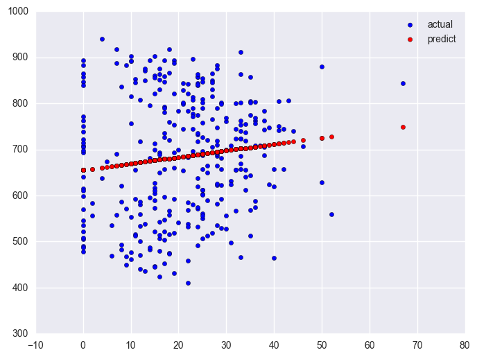
Say that we wish to analyze both continuous and categorical variables in one analysis. For example, let's include yr_rnd and some_col in the same analysis. We can also plot the predicted values against some_col using plot statement.
elemapi2_ = elemapi2.copy()

lm = smf.ols('api00 ~ yr_rnd + some_col', data = elemapi2_).fit()
print lm.summary()

elemapi2_['pred'] = lm.predict()

plt.scatter(elemapi2_.query('yr_rnd == 0').some_col, elemapi2_.query('yr_rnd == 0').pred, c = "b", marker = "o")
plt.scatter(elemapi2_.query('yr_rnd == 1').some_col, elemapi2_.query('yr_rnd == 1').pred, c = "r", marker = "+")
plt.plot()
                            OLS Regression Results
==============================================================================
Dep. Variable:                  api00   R-squared:                       0.257
Model:                            OLS   Adj. R-squared:                  0.253
Method:                 Least Squares   F-statistic:                     68.54
Date:                Sun, 22 Jan 2017   Prob (F-statistic):           2.69e-26
Time:                        14:27:31   Log-Likelihood:                -2490.8
No. Observations:                 400   AIC:                             4988.
Df Residuals:                     397   BIC:                             5000.
Df Model:                           2
Covariance Type:            nonrobust
==============================================================================
                 coef    std err          t      P>|t|      [95.0% Conf. Int.]
------------------------------------------------------------------------------
Intercept    637.8581     13.503     47.237      0.000       611.311   664.405
yr_rnd      -149.1591     14.875    -10.027      0.000      -178.403  -119.915
some_col       2.2357      0.553      4.044      0.000         1.149     3.323
==============================================================================
Omnibus:                       23.070   Durbin-Watson:                   1.565
Prob(Omnibus):                  0.000   Jarque-Bera (JB):                9.935
Skew:                           0.125   Prob(JB):                      0.00696
Kurtosis:                       2.269   Cond. No.                         62.5
==============================================================================

Warnings:
[1] Standard Errors assume that the covariance matrix of the errors is correctly specified.
The coefficient for some_col indicates that for every unit increase in some_col the api00 score is predicted to increase by 2.23 units. This is the slope of the lines shown in the above graph. The graph has two lines, one for the year round schools and one for the non-year round schools. The coefficient for yr_rnd is -149.16, indicating that as yr_rnd increases by 1 unit, the api00 score is expected to decrease by about 149 units. As you can see in the graph, the top line is about 150 units higher than the lower line. You can see that the intercept is 637 and that is where the upper line crosses the Y axis when X is 0. The lower line crosses the line about 150 units lower at about 487.
3.6.2 Using categorical variable directly
We can run this analysis using the categorical variable directly. We need to use the specify which variables should be considered as categorical variables.
lm = smf.ols('api00 ~ C(yr_rnd) + some_col', data = elemapi2_).fit()
print lm.summary()
                            OLS Regression Results
==============================================================================
Dep. Variable:                  api00   R-squared:                       0.257
Model:                            OLS   Adj. R-squared:                  0.253
Method:                 Least Squares   F-statistic:                     68.54
Date:                Sun, 22 Jan 2017   Prob (F-statistic):           2.69e-26
Time:                        14:29:38   Log-Likelihood:                -2490.8
No. Observations:                 400   AIC:                             4988.
Df Residuals:                     397   BIC:                             5000.
Df Model:                           2
Covariance Type:            nonrobust
==================================================================================
                     coef    std err          t      P>|t|      [95.0% Conf. Int.]
----------------------------------------------------------------------------------
Intercept        637.8581     13.503     47.237      0.000       611.311   664.405
C(yr_rnd)[T.1]  -149.1591     14.875    -10.027      0.000      -178.403  -119.915
some_col           2.2357      0.553      4.044      0.000         1.149     3.323
==============================================================================
Omnibus:                       23.070   Durbin-Watson:                   1.565
Prob(Omnibus):                  0.000   Jarque-Bera (JB):                9.935
Skew:                           0.125   Prob(JB):                      0.00696
Kurtosis:                       2.269   Cond. No.                         62.5
==============================================================================

Warnings:
[1] Standard Errors assume that the covariance matrix of the errors is correctly specified.
3.7 Interactions of Continuous by 0/1 Categorical variables
Above we showed an analysis that looked at the relationship between some_col and api00 and also included yr_rnd. We saw that this produced a graph where we saw the relationship between some_col and api00 but there were two regression lines, one higher than the other but with equal slope. Such a model assumed that the slope was the same for the two groups. Perhaps the slope might be different for these groups. Let's run the regressions separately for these two groups beginning with the non-year round schools.
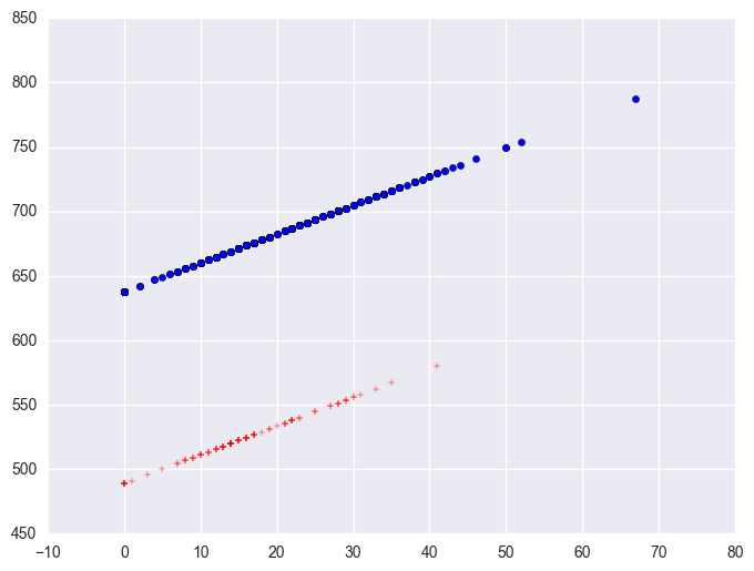
lm_0 = smf.ols(formula = "api00 ~ some_col", data = elemapi2.query('yr_rnd == 0')).fit()
lm_0.summary()
| Dep. Variable: | api00 | R-squared: | 0.016 |
|---|---|---|---|
| Model: | OLS | Adj. R-squared: | 0.013 |
| Method: | Least Squares | F-statistic: | 4.915 |
| Date: | Sun, 22 Jan 2017 | Prob (F-statistic): | 0.0274 |
| Time: | 09:43:46 | Log-Likelihood: | -1938.2 |
| No. Observations: | 308 | AIC: | 3880. |
| Df Residuals: | 306 | BIC: | 3888. |
| Df Model: | 1 | ||
| Covariance Type: | nonrobust |
| coef | std err | t | P>|t| | [95.0% Conf. Int.] | |
|---|---|---|---|---|---|
| Intercept | 655.1103 | 15.237 | 42.995 | 0.000 | 625.128 685.093 |
| some_col | 1.4094 | 0.636 | 2.217 | 0.027 | 0.158 2.660 |
| Omnibus: | 63.461 | Durbin-Watson: | 1.531 |
|---|---|---|---|
| Prob(Omnibus): | 0.000 | Jarque-Bera (JB): | 13.387 |
| Skew: | -0.003 | Prob(JB): | 0.00124 |
| Kurtosis: | 1.979 | Cond. No. | 48.9 |
plt.scatter(elemapi2.query('yr_rnd == 0').some_col.values, elemapi2.query('yr_rnd == 0').api00.values, label = "actual")
plt.scatter(elemapi2.query('yr_rnd == 0').some_col.values, lm_0.predict(), c = "r", label = "predict")
plt.legend()
plt.show()
Likewise, let's look at the year round schools and we will use the same symbol statements as above.
lm_1 = smf.ols(formula = "api00 ~ some_col", data = elemapi2.query('yr_rnd == 1')).fit()
plt.scatter(elemapi2.query('yr_rnd == 1').some_col.values, elemapi2.query('yr_rnd == 1').api00.values, label = "actual")
plt.scatter(elemapi2.query('yr_rnd == 1').some_col.values, lm_1.predict(), c = "r", label = "predict")
plt.legend()
plt.show()
Note that the slope of the regression line looks much steeper for the year round schools than for the non-year round schools. This is confirmed by the regression equations that show the slope for the year round schools to be higher (7.4) than non-year round schools (1.3). We can compare these to see if these are significantly different from each other by including the interaction of some_col by yr_rnd, an interaction of a continuous variable by a categorical variable.
3.7.1 Computing interactions manually
We will start by manually computing the interaction of some_col by yr_rnd.
Next, let's make a variable that is the interaction of some college (some_col) and year round schools (yr_rnd) called yrxsome.
yrxsome_elemapi = elemapi2
yrxsome_elemapi["yrxsome"] = yrxsome_elemapi.yr_rnd * yrxsome_elemapi.some_col
We can now run the regression that tests whether the coefficient for some_col is significantly different for year round schools and non-year round schools. Indeed, the yrxsome interaction effect is significant.
lm = smf.ols("api00 ~ some_col + yr_rnd + yrxsome", data = yrxsome_elemapi).fit()
lm.summary()
| Dep. Variable: | api00 | R-squared: | 0.283 |
|---|---|---|---|
| Model: | OLS | Adj. R-squared: | 0.277 |
| Method: | Least Squares | F-statistic: | 52.05 |
| Date: | Sun, 22 Jan 2017 | Prob (F-statistic): | 2.21e-28 |
| Time: | 09:48:54 | Log-Likelihood: | -2483.6 |
| No. Observations: | 400 | AIC: | 4975. |
| Df Residuals: | 396 | BIC: | 4991. |
| Df Model: | 3 | ||
| Covariance Type: | nonrobust |
| coef | std err | t | P>|t| | [95.0% Conf. Int.] | |
|---|---|---|---|---|---|
| Intercept | 655.1103 | 14.035 | 46.677 | 0.000 | 627.518 682.703 |
| some_col | 1.4094 | 0.586 | 2.407 | 0.017 | 0.258 2.561 |
| yr_rnd | -248.0712 | 29.859 | -8.308 | 0.000 | -306.773 -189.369 |
| yrxsome | 5.9932 | 1.577 | 3.800 | 0.000 | 2.893 9.094 |
| Omnibus: | 23.863 | Durbin-Watson: | 1.593 |
|---|---|---|---|
| Prob(Omnibus): | 0.000 | Jarque-Bera (JB): | 9.350 |
| Skew: | 0.023 | Prob(JB): | 0.00932 |
| Kurtosis: | 2.252 | Cond. No. | 117. |
We can then save the predicted values to a data set and graph the predicted values for the two types of schools by some_col. You can see how the two lines have quite different slopes, consistent with the fact that the yrxsome interaction was significant.
plt.scatter(yrxsome_elemapi.query('yr_rnd == 0').some_col, lm.predict()[yrxsome_elemapi.yr_rnd.values == 0], marker = "+")
plt.scatter(yrxsome_elemapi.query('yr_rnd == 1').some_col, lm.predict()[yrxsome_elemapi.yr_rnd.values == 1], c = "r", marker = "x")
<matplotlib.collections.PathCollection at 0x1107b780>
We can also create a plot including the data points. There are multiple ways of doing this and we'll show both ways and their graphs here.
plt.scatter(yrxsome_elemapi.query('yr_rnd == 0').some_col, lm.predict()[yrxsome_elemapi.yr_rnd.values == 0], marker = "+")
plt.scatter(yrxsome_elemapi.query('yr_rnd == 1').some_col, lm.predict()[yrxsome_elemapi.yr_rnd.values == 1], c = "r", marker = "x")
plt.scatter(yrxsome_elemapi.some_col, yrxsome_elemapi.api00, c = "black", marker = "*")
<matplotlib.collections.PathCollection at 0x1282cf98>
We can further enhance it so the data points are marked with different symbols. The graph above used the same kind of symbols for the data points for both types of schools. Let's make separate variables for the api00 scores for the two types of schools called api0 for the non-year round schools and api1 for the year round schools.
plt.scatter(yrxsome_elemapi.query('yr_rnd == 0').some_col, lm.predict()[yrxsome_elemapi.yr_rnd.values == 0], marker = "+")
plt.scatter(yrxsome_elemapi.query('yr_rnd == 1').some_col, lm.predict()[yrxsome_elemapi.yr_rnd.values == 1], c = "r", marker = "x")
plt.scatter(yrxsome_elemapi.query('yr_rnd == 0').some_col, yrxsome_elemapi.query('yr_rnd == 0').api00, c = "black", marker = "*")
plt.scatter(yrxsome_elemapi.query('yr_rnd == 1').some_col, yrxsome_elemapi.query('yr_rnd == 1').api00, c = "r", marker = "d")
<matplotlib.collections.PathCollection at 0x129dccf8>
Let's quickly run the regressions again where we performed separate regressions for the two groups. We first split data to yr_rnd = 0 group and yr_rnd = 1 group. Then run regression of api00 to some_col in each group seperately.
yrxsome_elemapi_0 = yrxsome_elemapi.query('yr_rnd == 0')
yrxsome_elemapi_1 = yrxsome_elemapi.query('yr_rnd == 1')


lm_0 = smf.ols("api00 ~ some_col", data = yrxsome_elemapi_0).fit()
print lm_0.summary()

print '\n'

lm_1 = smf.ols("api00 ~ some_col", data = yrxsome_elemapi_1).fit()
print lm_1.summary()
                            OLS Regression Results
==============================================================================
Dep. Variable:                  api00   R-squared:                       0.016
Model:                            OLS   Adj. R-squared:                  0.013
Method:                 Least Squares   F-statistic:                     4.915
Date:                Sun, 22 Jan 2017   Prob (F-statistic):             0.0274
Time:                        13:43:39   Log-Likelihood:                -1938.2
No. Observations:                 308   AIC:                             3880.
Df Residuals:                     306   BIC:                             3888.
Df Model:                           1
Covariance Type:            nonrobust
==============================================================================
                 coef    std err          t      P>|t|      [95.0% Conf. Int.]
------------------------------------------------------------------------------
Intercept    655.1103     15.237     42.995      0.000       625.128   685.093
some_col       1.4094      0.636      2.217      0.027         0.158     2.660
==============================================================================
Omnibus:                       63.461   Durbin-Watson:                   1.531
Prob(Omnibus):                  0.000   Jarque-Bera (JB):               13.387
Skew:                          -0.003   Prob(JB):                      0.00124
Kurtosis:                       1.979   Cond. No.                         48.9
==============================================================================

Warnings:
[1] Standard Errors assume that the covariance matrix of the errors is correctly specified.


                            OLS Regression Results
==============================================================================
Dep. Variable:                  api00   R-squared:                       0.420
Model:                            OLS   Adj. R-squared:                  0.413
Method:                 Least Squares   F-statistic:                     65.08
Date:                Sun, 22 Jan 2017   Prob (F-statistic):           2.97e-12
Time:                        13:43:39   Log-Likelihood:                -527.68
No. Observations:                  92   AIC:                             1059.
Df Residuals:                      90   BIC:                             1064.
Df Model:                           1
Covariance Type:            nonrobust
==============================================================================
                 coef    std err          t      P>|t|      [95.0% Conf. Int.]
------------------------------------------------------------------------------
Intercept    407.0391     16.515     24.647      0.000       374.230   439.848
some_col       7.4026      0.918      8.067      0.000         5.580     9.226
==============================================================================
Omnibus:                        5.042   Durbin-Watson:                   1.457
Prob(Omnibus):                  0.080   Jarque-Bera (JB):                4.324
Skew:                           0.471   Prob(JB):                        0.115
Kurtosis:                       3.492   Cond. No.                         37.7
==============================================================================

Warnings:
[1] Standard Errors assume that the covariance matrix of the errors is correctly specified.
Now, let's show the regression for both types of schools with the interaction term.
lm = smf.ols("api00 ~ some_col + yr_rnd + yrxsome", data = yrxsome_elemapi).fit()
lm.summary()
| Dep. Variable: | api00 | R-squared: | 0.283 |
|---|---|---|---|
| Model: | OLS | Adj. R-squared: | 0.277 |
| Method: | Least Squares | F-statistic: | 52.05 |
| Date: | Sun, 22 Jan 2017 | Prob (F-statistic): | 2.21e-28 |
| Time: | 13:43:29 | Log-Likelihood: | -2483.6 |
| No. Observations: | 400 | AIC: | 4975. |
| Df Residuals: | 396 | BIC: | 4991. |
| Df Model: | 3 | ||
| Covariance Type: | nonrobust |
| coef | std err | t | P>|t| | [95.0% Conf. Int.] | |
|---|---|---|---|---|---|
| Intercept | 655.1103 | 14.035 | 46.677 | 0.000 | 627.518 682.703 |
| some_col | 1.4094 | 0.586 | 2.407 | 0.017 | 0.258 2.561 |
| yr_rnd | -248.0712 | 29.859 | -8.308 | 0.000 | -306.773 -189.369 |
| yrxsome | 5.9932 | 1.577 | 3.800 | 0.000 | 2.893 9.094 |
| Omnibus: | 23.863 | Durbin-Watson: | 1.593 |
|---|---|---|---|
| Prob(Omnibus): | 0.000 | Jarque-Bera (JB): | 9.350 |
| Skew: | 0.023 | Prob(JB): | 0.00932 |
| Kurtosis: | 2.252 | Cond. No. | 117. |
Note that the coefficient for some_col in the combined analysis is the same as the coefficient for some_col for the non-year round schools? This is because non-year round schools are the reference group. Then, the coefficient for the yrxsome interaction in the combined analysis is the Bsome_col for the year round schools (7.4) minus Bsome_col for the non year round schools (1.41) yielding 5.99. This interaction is the difference in the slopes of some_col for the two types of schools, and this is why this is useful for testing whether the regression lines for the two types of schools are equal. If the two types of schools had the same regression coefficient for some_col, then the coefficient for the yrxsome interaction would be 0. In this case, the difference is significant, indicating that the regression lines are significantly different.
So, if we look at the graph of the two regression lines we can see the difference in the slopes of the regression lines (see graph below). Indeed, we can see that the non-year round schools (the solid line) have a smaller slope (1.4) than the slope for the year round schools (7.4). The difference between these slopes is 5.99, which is the coefficient for yrxsome.
plt.scatter(yrxsome_elemapi.query('yr_rnd == 0').some_col, lm.predict()[yrxsome_elemapi.yr_rnd.values == 0], marker = "+")
plt.scatter(yrxsome_elemapi.query('yr_rnd == 1').some_col, lm.predict()[yrxsome_elemapi.yr_rnd.values == 1], c = "r", marker = "x")
<matplotlib.collections.PathCollection at 0x12bba390>

3.7.2 Computing interactions with combinations
We can also run a model just like the model we showed above. We can include the terms yr_rnd some_col and the interaction yr_rnr*some_col.
lm = smf.ols("api00 ~ some_col + yr_rnd + yr_rnd * some_col ", data = yrxsome_elemapi).fit()
lm.summary()
| Dep. Variable: | api00 | R-squared: | 0.283 |
|---|---|---|---|
| Model: | OLS | Adj. R-squared: | 0.277 |
| Method: | Least Squares | F-statistic: | 52.05 |
| Date: | Sun, 22 Jan 2017 | Prob (F-statistic): | 2.21e-28 |
| Time: | 13:43:22 | Log-Likelihood: | -2483.6 |
| No. Observations: | 400 | AIC: | 4975. |
| Df Residuals: | 396 | BIC: | 4991. |
| Df Model: | 3 | ||
| Covariance Type: | nonrobust |
| coef | std err | t | P>|t| | [95.0% Conf. Int.] | |
|---|---|---|---|---|---|
| Intercept | 655.1103 | 14.035 | 46.677 | 0.000 | 627.518 682.703 |
| some_col | 1.4094 | 0.586 | 2.407 | 0.017 | 0.258 2.561 |
| yr_rnd | -248.0712 | 29.859 | -8.308 | 0.000 | -306.773 -189.369 |
| yr_rnd:some_col | 5.9932 | 1.577 | 3.800 | 0.000 | 2.893 9.094 |
| Omnibus: | 23.863 | Durbin-Watson: | 1.593 |
|---|---|---|---|
| Prob(Omnibus): | 0.000 | Jarque-Bera (JB): | 9.350 |
| Skew: | 0.023 | Prob(JB): | 0.00932 |
| Kurtosis: | 2.252 | Cond. No. | 117. |
In this section we found that the relationship between some_col and api00 depended on whether the school was from year round schools or from non-year round schools. For the schools from year round schools, the relationship between some_col and api00 was significantly stronger than for those from non-year round schools. In general, this type of analysis allows you to test whether the strength of the relationship between two continuous variables varies based on the categorical variable.
3.8 Continuous and categorical variables, interaction with 1/2/3 variable
The prior examples showed how to do regressions with a continuous variable and a categorical variable that has two levels. These examples will extend this further by using a categorical variable with three levels, mealcat.
3.8.1 Manually creating dummy variables
We can use a data step to create all the dummy variables needed for the interaction of mealcat and some_col just as we did before for mealcat. With the dummy variables, we can use regression for the regression analysis. We'll use mealcat1 as the reference group.
mxcol_elemapi = elemapi2
mxcol_elemapi["mealcat1"] = mxcol_elemapi.mealcat == 1
mxcol_elemapi["mealcat2"] = mxcol_elemapi.mealcat == 2
mxcol_elemapi["mealcat3"] = mxcol_elemapi.mealcat == 3
mxcol_elemapi["mxcol1"] = mxcol_elemapi.mealcat1 * mxcol_elemapi.some_col
mxcol_elemapi["mxcol2"] = mxcol_elemapi.mealcat2 * mxcol_elemapi.some_col
mxcol_elemapi["mxcol3"] = mxcol_elemapi.mealcat3 * mxcol_elemapi.some_col

lm = smf.ols("api00 ~ some_col + mealcat2 + mealcat3 +  mxcol2 + mxcol3", data = mxcol_elemapi).fit()
lm.summary()
| Dep. Variable: | api00 | R-squared: | 0.769 |
|---|---|---|---|
| Model: | OLS | Adj. R-squared: | 0.767 |
| Method: | Least Squares | F-statistic: | 263.0 |
| Date: | Sun, 22 Jan 2017 | Prob (F-statistic): | 4.13e-123 |
| Time: | 13:44:39 | Log-Likelihood: | -2256.6 |
| No. Observations: | 400 | AIC: | 4525. |
| Df Residuals: | 394 | BIC: | 4549. |
| Df Model: | 5 | ||
| Covariance Type: | nonrobust |
| coef | std err | t | P>|t| | [95.0% Conf. Int.] | |
|---|---|---|---|---|---|
| Intercept | 825.8937 | 11.992 | 68.871 | 0.000 | 802.318 849.470 |
| mealcat2[T.True] | -239.0300 | 18.665 | -12.806 | 0.000 | -275.725 -202.334 |
| mealcat3[T.True] | -344.9476 | 17.057 | -20.223 | 0.000 | -378.483 -311.413 |
| some_col | -0.9473 | 0.487 | -1.944 | 0.053 | -1.906 0.011 |
| mxcol2 | 3.1409 | 0.729 | 4.307 | 0.000 | 1.707 4.575 |
| mxcol3 | 2.6073 | 0.896 | 2.910 | 0.004 | 0.846 4.369 |
| Omnibus: | 1.272 | Durbin-Watson: | 1.565 |
|---|---|---|---|
| Prob(Omnibus): | 0.530 | Jarque-Bera (JB): | 1.369 |
| Skew: | -0.114 | Prob(JB): | 0.504 |
| Kurtosis: | 2.826 | Cond. No. | 177. |
The interaction now has two terms (mxcol2 and mxcol3). These results indicate that the overall interaction is indeed significant. This means that the regression lines from the three groups differ significantly. As we have done before, let's compute the predicted values and make a graph of the predicted values so we can see how the regression lines differ.
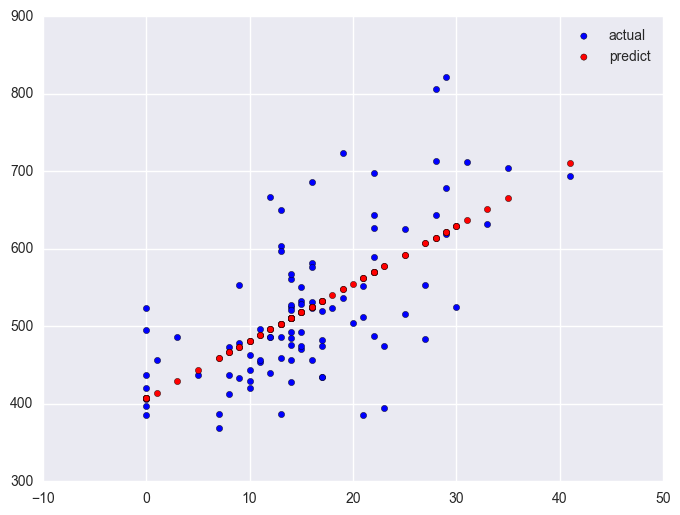
plt.scatter(mxcol_elemapi.query('mealcat == 1').some_col, lm.predict()[mxcol_elemapi.mealcat.values == 1], c = "black", marker = "+")
plt.scatter(mxcol_elemapi.query('mealcat == 2').some_col, lm.predict()[mxcol_elemapi.mealcat.values == 2], c = "red", marker = "+")
plt.scatter(mxcol_elemapi.query('mealcat == 3').some_col, lm.predict()[mxcol_elemapi.mealcat.values == 3], c = "b", marker = "+")
<matplotlib.collections.PathCollection at 0x144a4240>
Group 1 was the omitted group, therefore the slope of the line for group 1 is the coefficient for some_col which is -.94. Indeed, this line has a downward slope. If we add the coefficient for some_col to the coefficient for mxcol2 we get the coefficient for group 2, i.e., 3.14 + (-.94) yields 2.2, the slope for group 2. Indeed, group 2 shows an upward slope. Likewise, if we add the coefficient for some_col to the coefficient for mxcol3 we get the coefficient for group 3, i.e., 2.6 + (-.94) yields 1.66, the slope for group 3,. So, the slopes for the 3 groups are
group 1: -0.94
group 2:  2.2
group 3:  1.66
The test of the coefficient in the parameter estimates for mxcol2 tested whether the coefficient for group 2 differed from group 1, and indeed this was significant. Likewise, the test of the coefficient for mxcol3 tested whether the coefficient for group 3 differed from group 1, and indeed this was significant. What did the test of the coefficient some_col test? This coefficient represents the coefficient for group 1, so this tested whether the coefficient for group 1 (-0.94) was significantly different from 0. This is probably a non-interesting test.
The comparisons in the above analyses don't seem to be as interesting as comparing group 1 versus 2 and then comparing group 2 versus 3. These successive comparisons seem much more interesting. We can do this by making group 2 the omitted group, and then each group would be compared to group 2.
lm = smf.ols("api00 ~ some_col + mealcat1 + mealcat3 +  mxcol1 + mxcol3", data = mxcol_elemapi).fit()
lm.summary()
| Dep. Variable: | api00 | R-squared: | 0.769 |
|---|---|---|---|
| Model: | OLS | Adj. R-squared: | 0.767 |
| Method: | Least Squares | F-statistic: | 263.0 |
| Date: | Sun, 22 Jan 2017 | Prob (F-statistic): | 4.13e-123 |
| Time: | 13:52:16 | Log-Likelihood: | -2256.6 |
| No. Observations: | 400 | AIC: | 4525. |
| Df Residuals: | 394 | BIC: | 4549. |
| Df Model: | 5 | ||
| Covariance Type: | nonrobust |
| coef | std err | t | P>|t| | [95.0% Conf. Int.] | |
|---|---|---|---|---|---|
| Intercept | 586.8637 | 14.303 | 41.030 | 0.000 | 558.744 614.984 |
| mealcat1[T.True] | 239.0300 | 18.665 | 12.806 | 0.000 | 202.334 275.725 |
| mealcat3[T.True] | -105.9176 | 18.754 | -5.648 | 0.000 | -142.789 -69.046 |
| some_col | 2.1936 | 0.543 | 4.043 | 0.000 | 1.127 3.260 |
| mxcol1 | -3.1409 | 0.729 | -4.307 | 0.000 | -4.575 -1.707 |
| mxcol3 | -0.5336 | 0.927 | -0.576 | 0.565 | -2.357 1.289 |
| Omnibus: | 1.272 | Durbin-Watson: | 1.565 |
|---|---|---|---|
| Prob(Omnibus): | 0.530 | Jarque-Bera (JB): | 1.369 |
| Skew: | -0.114 | Prob(JB): | 0.504 |
| Kurtosis: | 2.826 | Cond. No. | 195. |
Now, the test of mxcol1 tests whether the coefficient for group 1 differs from group 2, and it does. Then, the test of mxcol3 tests whether the coefficient for group 3 significantly differs from group 2, and it does not. This makes sense given the graph and given the estimates of the coefficients that we have, that -.94 is significantly different from 2.2 but 2.2 is not significantly different from 1.66.
3.8.2 Using the combinations
We can perform the same analysis using the C and combinations directly as shown below. This allows us to avoid dummy coding for either the categorical variable mealcat and for the interaction term of mealcat and some_col. The tricky part is to control the reference group.
lm = smf.ols("api00 ~ some_col + C(mealcat) + some_col * C(mealcat)", data = mxcol_elemapi).fit()
lm.summary()
| Dep. Variable: | api00 | R-squared: | 0.769 |
|---|---|---|---|
| Model: | OLS | Adj. R-squared: | 0.767 |
| Method: | Least Squares | F-statistic: | 263.0 |
| Date: | Sun, 22 Jan 2017 | Prob (F-statistic): | 4.13e-123 |
| Time: | 13:53:55 | Log-Likelihood: | -2256.6 |
| No. Observations: | 400 | AIC: | 4525. |
| Df Residuals: | 394 | BIC: | 4549. |
| Df Model: | 5 | ||
| Covariance Type: | nonrobust |
| coef | std err | t | P>|t| | [95.0% Conf. Int.] | |
|---|---|---|---|---|---|
| Intercept | 825.8937 | 11.992 | 68.871 | 0.000 | 802.318 849.470 |
| C(mealcat)[T.2] | -239.0300 | 18.665 | -12.806 | 0.000 | -275.725 -202.334 |
| C(mealcat)[T.3] | -344.9476 | 17.057 | -20.223 | 0.000 | -378.483 -311.413 |
| some_col | -0.9473 | 0.487 | -1.944 | 0.053 | -1.906 0.011 |
| some_col:C(mealcat)[T.2] | 3.1409 | 0.729 | 4.307 | 0.000 | 1.707 4.575 |
| some_col:C(mealcat)[T.3] | 2.6073 | 0.896 | 2.910 | 0.004 | 0.846 4.369 |
| Omnibus: | 1.272 | Durbin-Watson: | 1.565 |
|---|---|---|---|
| Prob(Omnibus): | 0.530 | Jarque-Bera (JB): | 1.369 |
| Skew: | -0.114 | Prob(JB): | 0.504 |
| Kurtosis: | 2.826 | Cond. No. | 177. |
Because the default order for categorical variables is their numeric values, glm omits the third category. On the other hand, the analysis we showed in previous section omitted the second category, the parameter estimates will not be the same. You can compare the results from below with the results above and see that the parameter estimates are not the same. Because group 3 is dropped, that is the reference category and all comparisons are made with group 3.
These analyses showed that the relationship between some_col and api00 varied, depending on the level of mealcat. In comparing group 1 with group 2, the coefficient for some_col was significantly different, but there was no difference in the coefficient for some_col in comparing groups 2 and 3.
3.9 Summary
This chapter covered some techniques for analyzing data with categorical variables, especially, manually constructing indicator variables and using the categorical regression formula. Each method has its advantages and disadvantages, as described below.
Manually constructing indicator variables can be very tedious and even error prone. For very simple models, it is not very difficult to create your own indicator variables, but if you have categorical variables with many levels and/or interactions of categorical variables, it can be laborious to manually create indicator variables. However, the advantage is that you can have quite a bit of control over how the variables are created and the terms that are entered into the model.
The C formula approach eliminates the need to create indicator variables making it easy to include variables that have lots of categories, and making it easy to create interactions by allowing you to include terms like some_col * mealcat. It can be easier to perform tests of simple main effects. However, this is not very flexible in letting you choose which category is the omitted category.
As you will see in the next chapter, the regression command includes additional options like the robust option and the cluster option that allow you to perform analyses when you don't exactly meet the assumptions of ordinary least squares regression.
3.10 For more information
Reference