import numpy as np, pandas as pd
from matplotlib import pyplot as plt
import math
Gradient Descent is one of the optimization method by changing the parameters values in the negative gradient direction.
Let us assume the multi-variable function \(F(\theta|x)\) is differenable about \(\theta\). It is first order differentation to \(x\) is denoted as \(\triangledown F(\theta|x)\). To find the maximum(mimimum) of \(F(\theta|x)\) by iteration, we will let the parameter \(\theta\) change its value a little every time. The value changed along the gradient direction will be the fastest way to converge. So, from iteration \(\theta^{i}\) to iteration \(\theta^{i+1}\) we will let
where \(\lambda\) is called learning rate.
In the following two examples will be shown how gradient descent works to find the solution: one is for linear regression(which has closed-form solution) and the other is for logistic regression(which does not have closed-form solution).


Example 1: Linear regression
A simple example of linear regression function can be written as
we can write it in vector form as
where
The target is to minimize the Mean Square Error(mse) function defined as
We will call its main part Loss function :
As introducted above, the gradient of the loss function to the parameter \(W\) is:
Now we will show how to use this gradient to find the final value of \(W\).
ns = 100
x = np.c_[np.ones(ns), np.linspace(0, 10, ns)]
y = x.dot([[3], [8]]) + np.random.normal(0, 1, ns).reshape(-1, 1)

def loss(w):
    e = y - x.dot(w)
    return e.T.dot(e)
The initial value of \(W\) will be
For each loop,
w0 = np.array([0.0, 0.0]).reshape(2, 1)
learning_rate = 0.00001

i = 0
w = w0
while True:
    l1 = loss(w)
    dldw = -2 * x.T.dot(y - x.dot(w))
    w_new = w - dldw * learning_rate
    l2 = loss(w_new)
    w = w_new
    i += 1
    if i > 10000 or abs(l1 - l2) < 0.00001:
        break

print("The final value from gradient descent is alpha_0 = %.2f, alpha_1 = %.2f" %(w[0], w[1]))
The final value from gradient descent is alpha_0 = 2.41, alpha_1 = 8.09
For linear regression, we have the analytical solution(or closed-form solution) in the form:
So the analytical solution can be calculated directly in python. The analytical solution is: constant = 2.73 and the slope is 8.02.
regres = np.linalg.inv((x.T.dot(x))).dot(x.T.dot(y))
print("The regression result is alpha_0 = {0:.2f}, alpha_1 = {1:.2f}".format(round(regres[0], 2), round(regres[1], 2)))
The regression result is alpha_0 = 2.43, alpha_1 = 8.09
Logistic Regression
Random variable \(Y\) has Bernoulli distribution:
Here \(p\) is the function of \(X\) given parameters \(W\): \(p = p(X|W)\).
The logit function is
here both \(X\) and \(W\) are vectors(shall be written as \(\vec{X}\) and \(\vec{W}\))
So the likelihood funciton can be written as
To max the likelihood function is the same as maximizing the log-likelihood funtion. The log-likelihood function is
from this we can get the gradient of \(W\) is
where
Next an example is shown how to use gradient descent to find the solution of \(W\) to maximize the likelihood function.The link function is of the form:
w = np.array([1, 2, 5]).reshape(3, 1)
np.random.seed(99)
x = np.c_[np.ones(100).reshape(100, 1), np.random.normal(0, 2, 200).reshape(100, 2)]
s = x.dot(w) + np.random.normal(0, 1, 100).reshape(100, 1)
p = np.exp(s) / (1 + np.exp(s))
y = np.random.binomial(1, p).reshape(100, 1)
def sgd(x, y, w):
    expval = np.exp(x[:, :].dot(w))
    return np.sum([expval / (1 + expval) - y] * x, axis = 1).reshape(3, -1)
w0 = np.zeros(3).reshape(3, 1)
learning_rate = 0.01
i = 0
w = w0
while True:
dlldw = sgd(x, y, w)
w_new = w - dlldw * learning_rate
i += 1
if i > 1000 or sum((w - w_new)**2)<0.00001:
break
w = w_new
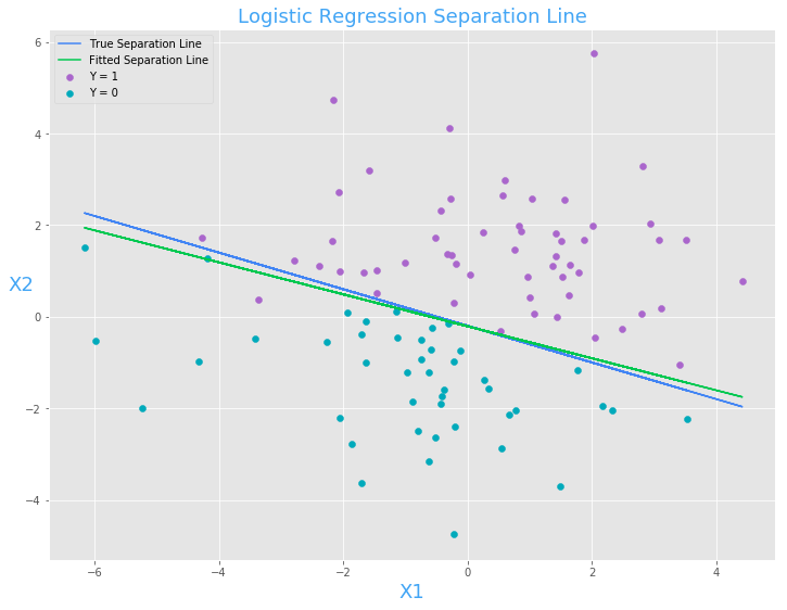
print("The fitting result from gradient descent is beta0 = %.2f, beta1 = %.2f, beta2 = %.2f" %(w[0], w[1], w[2]))
The fitting result from gradient descent is beta0 = 1.09, beta1 = 1.82, beta2 = 5.20
plt.scatter(x[y.reshape(100, ) ==1, 1], x[y.reshape(100, ) ==1, 2], color = "#aa66cc", label = "Y = 1")
plt.scatter(x[y.reshape(100, ) ==0, 1], x[y.reshape(100, ) ==0, 2], color = "#00aabb", label = "Y = 0")
plt.plot(x[:, 1], -0.2 - 0.4 * x[:, 1], color = "#4285F4", label = "True Separation Line")
plt.plot(x[:, 1], -x[:, :2].dot(w[:2, 0] / w[2, 0]), color = "#00C851", label = "Fitted Separation Line")
plt.xlabel("X1", color = '#42a5f5', size = "18")
h = plt.ylabel('X2', color = '#42a5f5', size = "18")
h.set_rotation(0)
plt.title("Logistic Regression Separation Line", color = "#42a5f5", size = "18")
plt.legend(loc=2)
The same as linear regression, we can use sklearn(it also use gradient method to solve) or statsmodels(it is the same as traditional method like R or SAS did) to get the regression result for this example:
from sklearn.linear_model import LogisticRegression
logfit = LogisticRegression()
logfit.fit(x, y)
sklearn_w = logfit.coef_[0]
print("The fitting result from gradient descent is beta0 = %.2f, beta1 = %.2f, beta2 = %.2f" %(sklearn_w[0], sklearn_w[1], sklearn_w[2]))

# import statsmodels.formula.api as smf
# import statsmodels.api as sm
# import pandas as pd
# mydata = pd.DataFrame(np.c_[x, y], columns = ["const", "x1", "x2", "y"])
# mod1 = smf.glm(formula = "y ~ x1 + x2", data=mydata, family=sm.families.Binomial()).fit()
# print (mod1.params)
The fitting result from gradient descent is beta0 = 0.27, beta1 = 0.95, beta2 = 2.72