The previous notes introduced the text generation models (GPT family). This reading note is about image generator papers.
Similar to text generator which generate the next token, OpenAI has image-GPT which is a large transformer trained on next pixel prediction in which the pixels are concated into a vector to build the autoregressive model. This model is time consuming as one image has lots of pixels compared to the tokens in the sentence.
Other models usually generate image from an embedding vector rather than pixel by pixel. These generative models usually have the input from the probability distribution (e.g., normal distribution). The sample vector is put into the image generator model to generate the image. These models include: 1) VAE; 2) Flow-based models; 3) GAN and 4) Diffusion models.
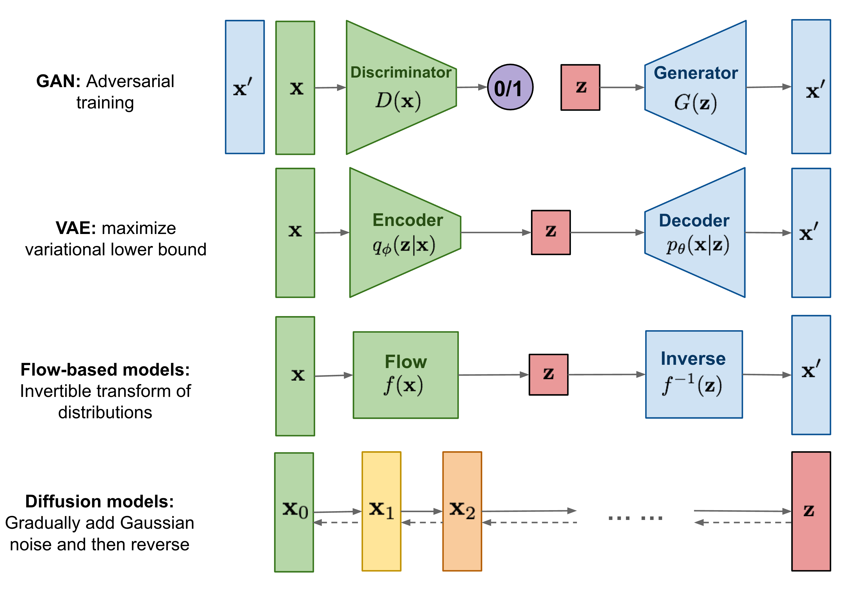
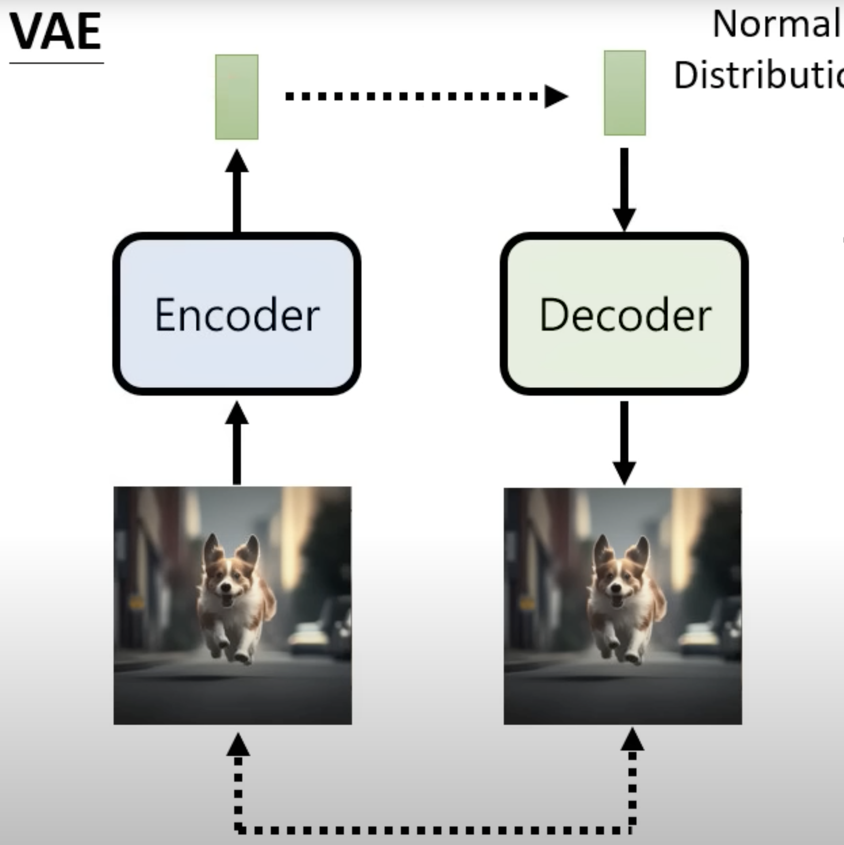
VAE: VAE had an encoder to convert the input image to a vector and the decoder model to convert the vector (normal distribution) to image.
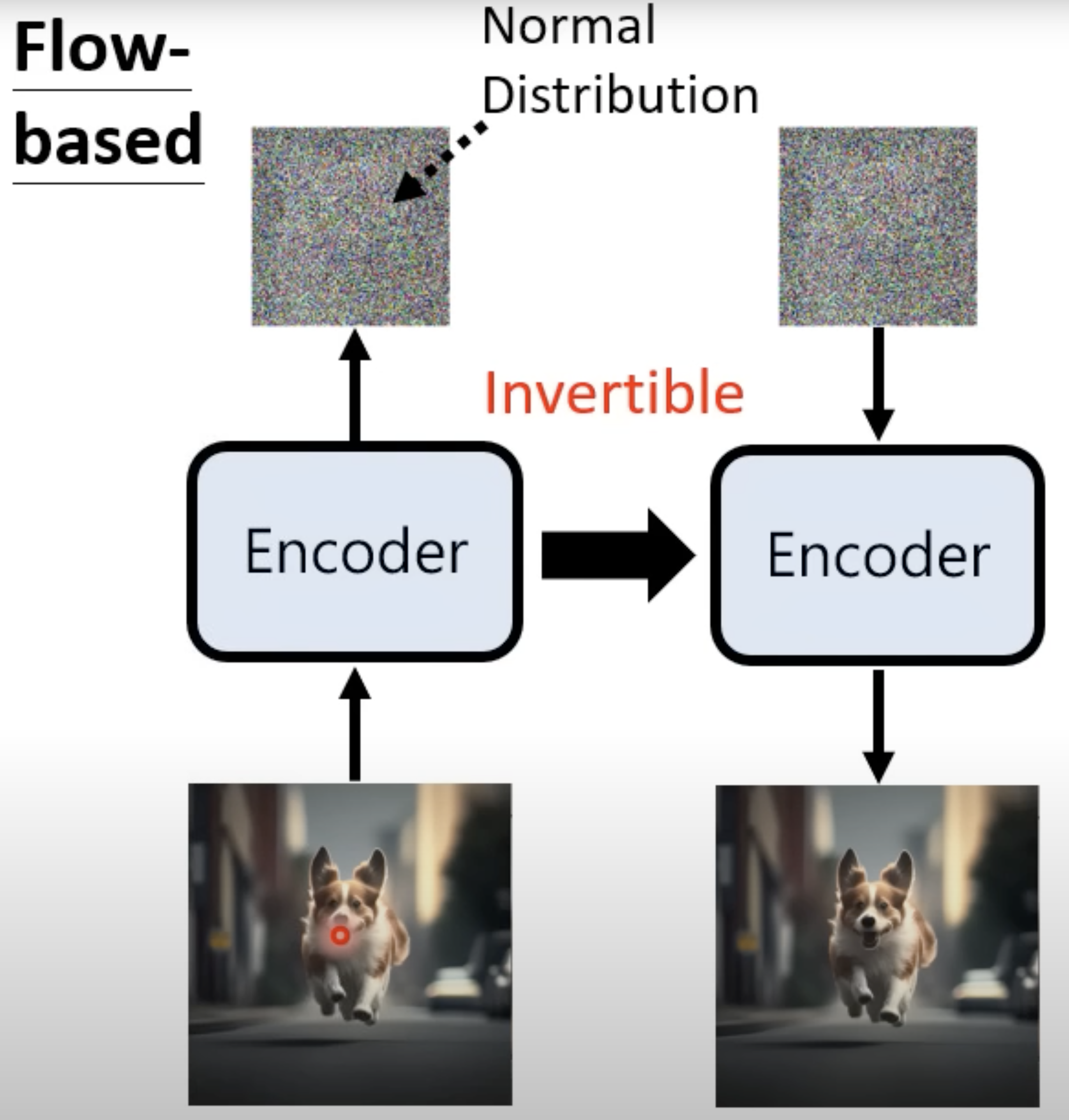
Flow-based model: it trains an encoder model to convert the input image to a vector (normally distributed) and the encoder is invertible that can be used to convert the vector to image. To make the encoder invertible, the input and the output of the encoder mush have the same size.
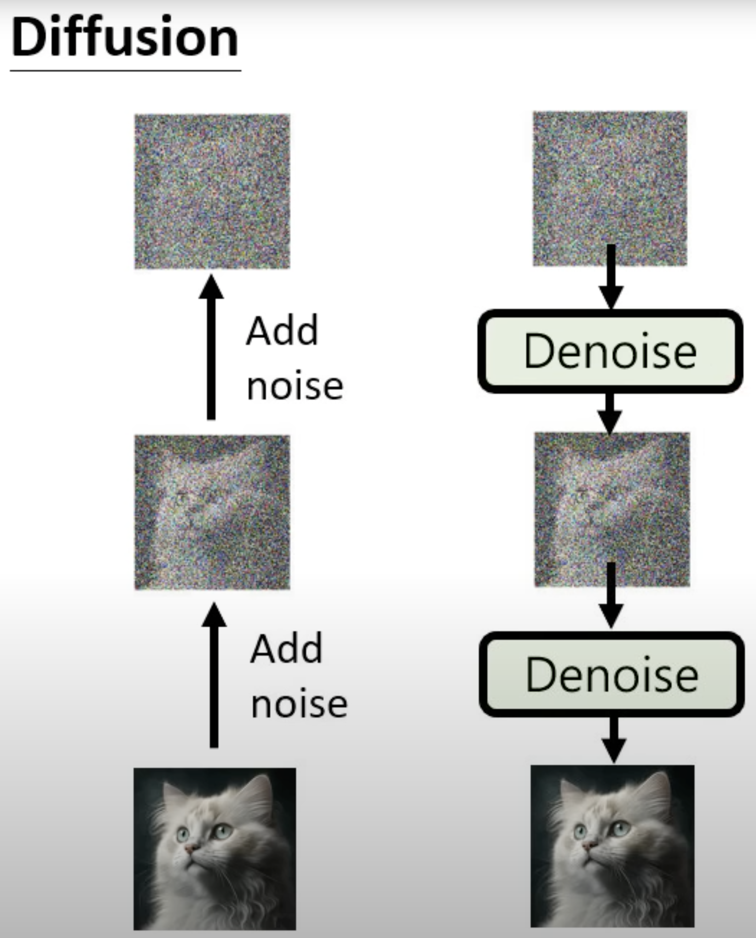
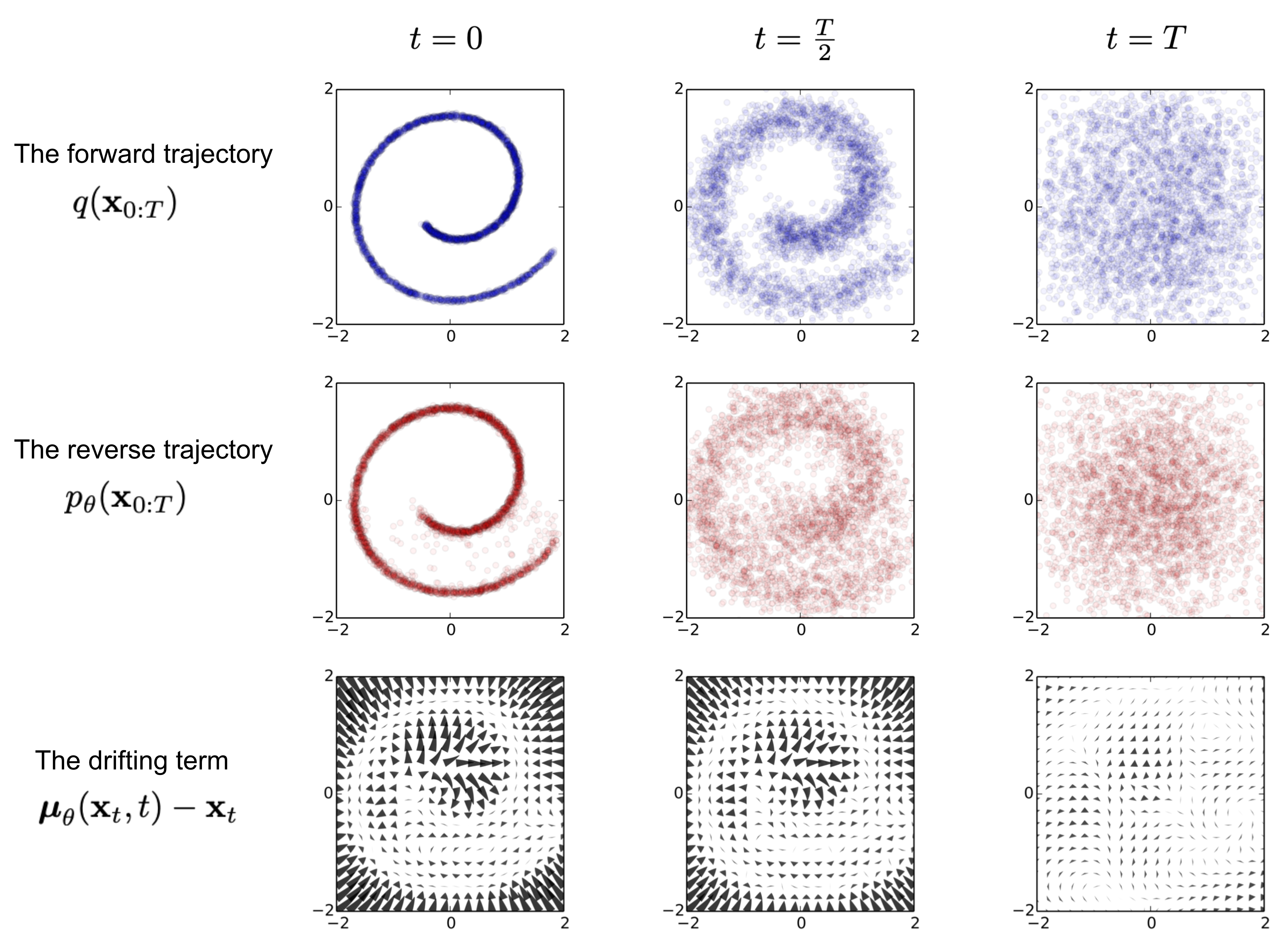
Diffusion model: diffusion model has the forward diffusion process that gradually adds Gaussian noise to an image until the image converge to Gaussian noise, and the reverse diffusion process where a neural network is trained to denoise from the Gaussian noise to an image.
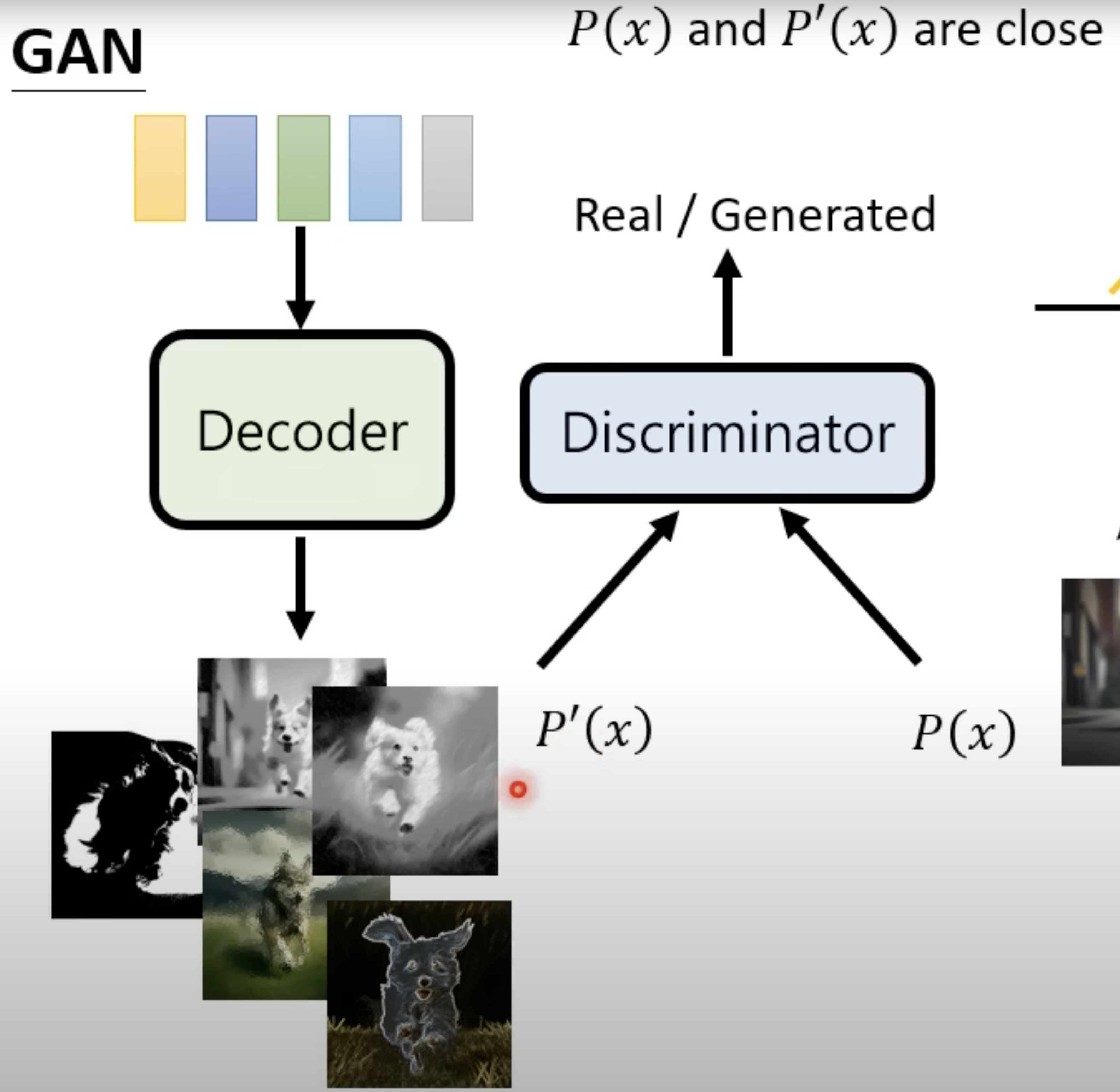
GAN: GAN consists of two simultaneously trained model, one is Generator trained to generate fake data and the other is Discriminator trained to discriminate the fake data from the real data.
| Generative Models | |
|---|---|
 |
 |
 |
 |
As most of the text to image generative models like DALLE2, ImageGen, CLIP are all based on the diffusion model, we will start from the diffusion model.
What are Diffusion Models?
Diffusion Models include two steps: the first step is to add noice to the image step by step to convert the image to white noise, which is called Forward Diffusion Process; the second is to denoise from the white noise back to the image, which is called Reverse Diffusion Process.
Forward diffusion process
Given a data \(\mathbf{x}_0\) sampled from the data distribution \(\mathbf{x}_0 \sim q(\mathbf{x})\), forward diffusion process is to add a small amount of white noise to it in \(1, 2, \cdots, T\) steps to produce the sequence \(\mathbf{x}_1, \mathbf{x}_2, \cdots, \mathbf{x}_T\). From step \(t-1\) to step \(t\), the input is degraded by \(\sqrt{1-\beta_t}\) and the new added noise is \(\sqrt{\beta_t} \boldsymbol{\epsilon}_{t-1}\) where \(\beta_t \in (0, 1)\) and \(\boldsymbol{\epsilon}_{t-1} \sim \mathcal{N}(0, \mathbf{I})\), that is \(\mathbf{x}_t = \sqrt{1-\beta_t} \mathbf{x}_{t-1} + \sqrt{\beta_t} \boldsymbol{\epsilon}_{t-1}\). In the experiment, the varience in each step is set to linearly increasing from \(\beta_1 = 10^{-5}\) to \(\beta_T = 0.02\). Based on the relation from \(\mathbf{x}_t\) to \(\mathbf{x}_{t-1}\), we can deduce the relation of \(\mathbf{x}_{t-1}\) to \(\mathbf{x}_{t-2}\) and replace \(\mathbf{x}_{t-1}\) with \(\mathbf{x}_{t-2}\), and so on. After the iteration until \(\mathbf{x}_{0}\), we have the relation of \(\mathbf{x}_{t}\) represented as \(\mathbf{x}_{0}\):
where \(\alpha_t = 1 - \beta_t\) and \(\bar{\alpha}_t = \prod_{s=1}^t \alpha_s\).
In python:
    alpha = 1. - beta
    alpha_hat = torch.cumprod(alpha, dim=0)
    sqrt_alpha_hat = torch.sqrt(alpha_hat[t])[:, None, None, None]
    sqrt_one_minus_alpha_hat = torch.sqrt(1 - alpha_hat[t])[:, None, None, None]
    z = torch.randn_like(x)
    sqrt_alpha_hat * x + sqrt_one_minus_alpha_hat * z
Reverse diffusion process
This step is also called denoise as it is from the noise \(\mathbf{x}_{T}\) back to the image \(\mathbf{x}_{0}\), like from \(\mathbf{x}_{T} \rightarrow \mathbf{x}_{t-1} \rightarrow \cdots \rightarrow \mathbf{x}_{1} \rightarrow \mathbf{x}_{0}\). That is, given \(\mathbf{x}_{t}\), this step is to find a noise term \(\boldsymbol{\epsilon}_t\) so that \(\mathbf{x}_{t-1} = \mathbf{x}_{t} - \boldsymbol{\epsilon}_t\), Theoretially this is not doable as you need to start from the white noise \(\mathbf{x}_{T}\) to get an image \(\mathbf{x}_{0}\) by denoising. But is there any way to get \(q(\mathbf{x}_{t-1} | \mathbf{x}_{t})\)? We can rewrite it based on Bayesian formula
In this way we convert \(q(\mathbf{x}_{t-1} \vert \mathbf{x}_t)\) to \(q(\mathbf{x}_t \vert \mathbf{x}_{t-1}), q(\mathbf{x}_{t-1}), \text{ and } q(\mathbf{x}_t)\). The thing is, we still don't know \(q(\mathbf{x}_{t-1}) \text{ and } q(\mathbf{x}_t)\). But we know \(q(\mathbf{x}_{t-1} \vert \mathbf{x}_0)\) from fowward process. So now we will rewrite the formula to conditional on \(\mathbf{x}_0\), and denote it as \(q(\mathbf{x}_{t-1} \vert \mathbf{x}_t, \mathbf{x}_0)\). That is, we want to calculate \(\color{blue} {q(\mathbf{x}_{t-1} \vert \mathbf{x}_t, \mathbf{x}_0)}\).
From the forward process, we know that:
From the Bayesian formula, we have:
This is the kernel funciton for normal distribution with the mean equals to:
Here \(\boldsymbol{\epsilon}_t\) is not known, it will be learned from the forward process. In forward process, from \(\mathbf{x}_t\) to \(\mathbf{x}_{t+1}\) by adding a noise \(\boldsymbol{\epsilon}_t\). The true value is from the difference of the input, and A NN model (in the paper, it is UNet) will be built to learn this added noice.
In python:
    predicted_noise = model(x, t)
    x = 1 / torch.sqrt(alpha) * (x - ((1 - alpha) / (torch.sqrt(1 - alpha_hat))) * predicted_noise) + torch.sqrt(beta) * noise
Algorithm

Training: Combine the forward and reverse process together, in the training process, step \(t\) in the forward process will generate the true value of the noise for that given step, and the reverse process will try to build a neural network model to predict the denoised term, which should be close to the noise term in the froward process. Because for any step \(t\), it needs to learn the noise so the step \(t\) will also be an input to the model.
In all, there are two inputs to the initial step: a given image \(\mathbf{x}_{0}\) and the step \(t\). It will learn a neural network (U-net in the original paper) \(\boldsymbol{\epsilon}_{\theta}\) to approxiate the added Gaussian noise where \(\boldsymbol{\epsilon}_{\theta} = \boldsymbol{\epsilon}_{\theta}\left(\sqrt{\bar{\alpha}_t}\mathbf{x}_0 + \sqrt{1 - \bar{\alpha}_t}\boldsymbol{\epsilon}, t \right)\).
Sampling: starting from the Gaussian noise \(\mathbf{x}_{T} \sim \mathcal{N}(0, \mathbf{I})\), for each step \(t\), calculate the denoised term from the trained neural network \(\boldsymbol{\epsilon}_{\theta}(\mathbf{x}_{t}, t)\) and then denoise from step \(t\) to step \(t-1\) through \(\mathbf{x}_{t-1} = {\frac{1}{\sqrt{\alpha_t}} \Big( \mathbf{x}_t - \frac{1 - \alpha_t}{\sqrt{1 - \bar{\alpha}_t}} \boldsymbol{\epsilon}_{\theta}(\mathbf{x}_t, t) \Big)} + \sigma_t \mathbf{z}\) where \(\mathbf{z}\) is Gaussian noise for \(t>1\) else 0.