Tensorflow简介--06: Logistic regression and KNN analysis for MNIST data

import numpy as np
import matplotlib.pyplot as plt
import tensorflow as tf

from tensorflow.examples.tutorials.mnist import input_data
mnist = input_data.read_data_sets("MNIST_data/", one_hot=True)

Data Introduction

The backgroupnd of MNIST data is introduced in MNIST For ML Beginners

The MNIST data is split into three parts: 55,000 data points of training data (mnist.train), 10,000 points of test data (mnist.test), and 5,000 points of validation data (mnist.validation). This split is very important: it's essential in machine learning that we have separate data which we don't learn from so that we can make sure that what we've learned actually generalizes!

the training images are mnist.train.images and the training labels are mnist.train.labels.

Each image is 28 pixels by 28 pixels. We can interpret this as a big array of numbers. We can flatten this array into a vector of 28x28 = 784 numbers.

The result is that mnist.train.images is a tensor (an n-dimensional array) with a shape of [55000, 784]. The first dimension is an index into the list of images and the second dimension is the index for each pixel in each image. Each entry in the tensor is a pixel intensity between 0 and 1, for a particular pixel in a particular image.

Each image in MNIST has a corresponding label, a number between 0 and 9 representing the digit drawn in the image.

For the purposes of this tutorial, we're going to want our labels as "one-hot vectors". A one-hot vector is a vector which is 0 in most dimensions, and 1 in a single dimension. In this case, the nth digit will be represented as a vector which is 1 in the nth dimension. For example, 3 would be $[0,0,0,1,0,0,0,0,0,0]$. Consequently, mnist.train.labels is a [55000, 10] array of floats.

1. Softmax Regressions (multinomial logistic regression)

Here is an introduction of Softmax Regression. It is a multivariate logistic regression.

$$ \begin{aligned} & \text{evidence}_i = \sum_j W_{i,~ j} x_j + b_i \\\ & y = \text{softmax}(\text{evidence}) \\\ & \text{softmax}(x) = \text{normalize}(\exp(x)) \\\ & \text{softmax}(x)_i = \frac{\exp(x_i)}{\sum_j \exp(x_j)} \end{aligned} $$

Implementation

First we will define the input data.

init_param = lambda shape: tf.random_normal(shape, dtype=tf.float32)

with tf.name_scope("IO"):
    inputs = tf.placeholder(tf.float32, [None, 784], name="X")
    targets = tf.placeholder(tf.float32, [None, 10], name="Yhat")

As explained above, Input data(training data x) is the array with shape of [55000, 784]. The target variable shape is [55000, 10]. placeholder: a value that we'll input when we ask TensorFlow to run a computation. It will enable you to assemble the graph first without knowing the values needed for computation. In the computation, you can feed the values to placeholders using a dictionary. None means that a dimension can be of any length.

Next we will define the variables in the model.

Variable is a modifiable tensor that lives in TensorFlow's graph of interacting operations. tf.Variable is a class, but tf.constant is an operation. tf.Variable also hold some operations lile assign. tf.Variable must be initialized and can be evaluated to get the values.

with tf.name_scope("LogReg"):
    W = tf.Variable(init_param([784, 10]), name="W")
    B = tf.Variable(init_param([10]))
    logits = tf.matmul(inputs, W) + B
    y = tf.nn.softmax(logits)

Then we will define the loss function. The purpose it to optimize(minimize) the loss function to find the value of the parameters defined as variables.

with tf.name_scope("train"):
    learning_rate = tf.Variable(0.5, trainable=False)
    cost_op = tf.nn.softmax_cross_entropy_with_logits(logits = logits, labels = targets)
    cost_op = tf.reduce_mean(cost_op) 
    train_op = tf.train.GradientDescentOptimizer(learning_rate).minimize(cost_op)

    correct_prediction = tf.equal(tf.argmax(y, 1), tf.argmax(targets,1))
    accuracy = tf.reduce_mean(tf.cast(correct_prediction, tf.float32))*100

Finally is to loop through the epochs to minimize the loss function. The iteration will stop when it reaches the stoping condition or the max of epoch.

Sometimes the input data will be very big(considering training the pictures with CNN in computer vision / object recognizatio). If dump all data into memory, it will cause the system crashed unless you have lots of ram installed. To avoid this, the best way is to split the input into different batches, then read in and train each batch. Please refer to tensorflow--02 for the details how batch and mini-batch works.

tolerance = 1e-4
epochs = 1
last_cost = 0.0
alpha = 0.5
max_epochs = 10
batch_size = 100
costs = []
sess = tf.Session()

with sess.as_default():
    init = tf.global_variables_initializer()
    sess.run(init)
    sess.run(tf.assign(learning_rate, alpha))
    writer = tf.summary.FileWriter("./tfboard", sess.graph)
    while True:

        num_batches = int(mnist.train.num_examples/batch_size)
        cost=0
        for _ in range(num_batches):
            batch_xs, batch_ys = mnist.train.next_batch(batch_size)
            tcost, _ = sess.run([cost_op, train_op], feed_dict={inputs: batch_xs, targets: batch_ys})
            cost += tcost
        cost /= num_batches

        tcost = sess.run(cost_op, feed_dict={inputs: mnist.test.images, targets: mnist.test.labels})
        costs.append([cost, tcost])

        if epochs%5==0:
            acc = sess.run(accuracy, feed_dict={inputs: mnist.train.images, targets: mnist.train.labels})
            print ("Epoch: %d - Error: %.4f - Accuracy - %.2f%%" %(epochs, cost, acc))

            if abs(last_cost - cost) < tolerance or epochs > max_epochs:
                break

            last_cost = cost

        epochs += 1

    tcost, taccuracy = sess.run([cost_op, accuracy], feed_dict={inputs: mnist.test.images, targets: mnist.test.labels})
    print ("Test Cost: %.4f - Accuracy: %.2f%% " %(tcost, taccuracy))
    test_plot = sess.run(tf.argmax(y, 1), feed_dict = {inputs: mnist.test.images[:9]})

Epoch: 5 - Error: 0.4307 - Accuracy - 89.50%
Epoch: 10 - Error: 0.3502 - Accuracy - 91.15%
Epoch: 15 - Error: 0.3164 - Accuracy - 91.91%
Test Cost: 0.3292 - Accuracy: 91.27%

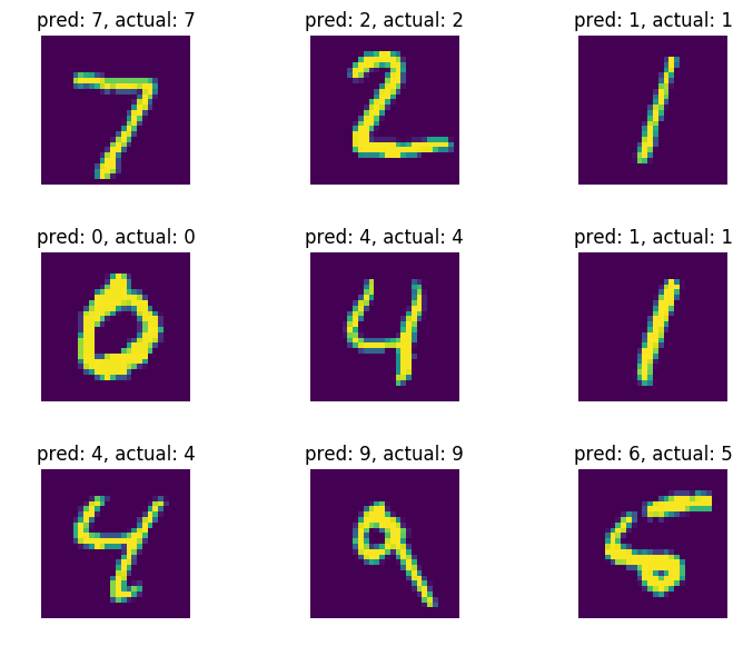
%matplotlib inline
fig = plt.figure(dpi=100, figsize=(9, 6))
labels = np.argmax(mnist.test.labels[:9], axis = 1)
for i in range(9):
    fig.add_subplot(3, 3, i+1)
    plt.imshow(mnist.test.images[i].reshape(28, 28))
    plt.axis("off")
    plt.tight_layout()
    plt.title("pred: " + str(test_plot[i]) + ', actual: ' + str(labels[i]))
    #frame = plt.gca()
    #frame.axes.get_xaxis().set_visible(False)
    #frame.axes.get_yaxis().set_visible(False)

plt.show()

png

2. KNN

KNN is a non-parametric method for classification and regression. It will measure the distance and group the k nearest data together for classification or regression.

A common used distance is Euclidean distance given by

$$ d(x, x')=\sqrt{(x_1 − x′_1)^2+(x_2−x′_2)^2+ \cdots +(x_n−x′_n)^2} $$

More formally, given a positive integer $K$, an unseen observation $x$ and a similarity metric $d$, KNN classifier performs the following two steps:

1, It runs through the whole dataset computing $d$ between $x$ and each training observation. We’ll call the $K$ points in the training data that are closest to $x$ the set $\mathcal{A}$. Note that $K$ is usually odd to prevent tie situations.

2, It then estimates the conditional probability for each class, that is, the fraction of points in $\mathcal{A}$ with that given class label. (Note $I(x)$ is the indicator function which evaluates to 1 when the argument $x$ is true and 0 otherwise)

$$ P(y = j | X = x) = \frac{1}{K} \sum_{i \in \mathcal{A}} I(y^{(i)} = j) $$

Finally, our input $x$ gets assigned to the class with the largest probability.

sess = tf.Session()


np.random.seed(13)  # set seed for reproducibility
train_size = 2000
test_size = 200
rand_train_indices = np.random.choice(len(mnist.train.images), train_size, replace=False)
rand_test_indices = np.random.choice(len(mnist.test.images), test_size, replace=False)
x_vals_train = mnist.train.images[rand_train_indices]
x_vals_test = mnist.test.images[rand_test_indices]
y_vals_train = mnist.train.labels[rand_train_indices]
y_vals_test = mnist.test.labels[rand_test_indices]

k = 5
batch_size=5

with tf.name_scope("IO"):
# Placeholders
    x_data_train = tf.placeholder(shape=[None, 784], dtype=tf.float32)
    x_data_test = tf.placeholder(shape=[None, 784], dtype=tf.float32)
    y_target_train = tf.placeholder(shape=[None, 10], dtype=tf.float32)
    y_target_test = tf.placeholder(shape=[None, 10], dtype=tf.float32)

with tf.name_scope("KNN"):    
    #each train and each test dist
    distance = tf.reduce_sum(tf.abs(tf.subtract(x_data_train, tf.expand_dims(x_data_test,1))), axis=2) 
    # Get min distance index (Nearest neighbor)
    top_k_xvals, top_k_indices = tf.nn.top_k(tf.negative(distance), k=k)
    prediction_indices = tf.gather(y_target_train, top_k_indices)
    # Predict the mode category: k nearest nbrs may result in different preds, pick the pred with highest freq
    count_of_predictions = tf.reduce_sum(prediction_indices, axis=1)
    prediction = tf.argmax(count_of_predictions, axis=1)


num_loops = int(np.ceil(len(x_vals_test)/batch_size))
test_output = []
actual_vals = []

with sess.as_default():
    for i in range(num_loops):
        init = tf.global_variables_initializer()
        sess.run(init)
        min_index = i*batch_size
        max_index = min((i+1)*batch_size,len(x_vals_train))
        x_batch = x_vals_test[min_index:max_index] 
        y_batch = y_vals_test[min_index:max_index]
        predictions = sess.run(prediction, feed_dict={x_data_train: x_vals_train, x_data_test: x_batch,
                                             y_target_train: y_vals_train, y_target_test: y_batch})
        test_output.extend(predictions)
        actual_vals.extend(np.argmax(y_batch, axis=1))

    accuracy = sum([1./test_size for i in range(test_size) if test_output[i]==actual_vals[i]])
    print("Accuracy on test data: %.2f%% " %(accuracy))

Accuracy on test data: 0.87%

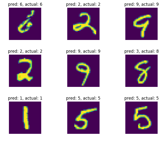
%matplotlib inline
fig = plt.figure(dpi=100, figsize=(9, 6))


for i in range(9):
    fig.add_subplot(3, 3, i+1)
    plt.imshow(x_vals_test[:9][i].reshape(28, 28))
    plt.axis("off")
    plt.tight_layout()
    plt.title("pred: " + str(test_output[:9][i]) + ', actual: ' + str(actual_vals[:9][i]))

plt.show()

png

broadcasting

the dimension of xtrain and xtest are different. so the substraction cannot be applied directly. tf.expand_dims(x_vals_test,1) will add one dimension on the data. After expanding the dim, the substraction is fine becasue of broadcasting. It is the same as np.expand_dim. An example is given below.

import numpy as np
x = np.arange(100).reshape(20, 5)  # 20x5
y = np.arange(20).reshape(4, 5)    # 4x5
x - y # error

print (np.expand_dims(y, 1).shape)        # 4x1x5
print((x  - np.expand_dims(y, 1)).shape)  # 4x20x5
print(np.sum(np.abs((x  - np.expand_dims(y, 1))), axis = 2).shape)    # 4x20

(4, 1, 5)
(4, 20, 5)
(4, 20)

tf.reduce_sum(, axis = 2) will calculate the sum on the given axis = 2. It is similar to np.sum(, axis = 2)

np.random.seed(99)
float_formatter = lambda x: "%.2f" % x

s = np.round(np.random.normal(0, 1, 10), 2) 
#s = np.array(map(float_formatter, s))

print s

print(-s[np.argsort(-s)[::-1][:2]])

with tf.Session() as sess:
    sess.run(init)
    print sess.run(tf.nn.top_k(tf.negative(s), k=2))

[-0.14  2.06  0.28  1.33 -0.15 -0.07  0.76  0.83 -0.11 -2.37]

[ 2.37  0.15]

TopKV2(values=array([ 2.37,  0.15]), indices=array([9, 4], dtype=int32))

pydata

Keep Looking, Don't Settle