1. Prediciton in Decoder

在前面GPT summary里面对GPT的模型有一个综合的介绍，这里用一个fake example来解释一步步GPT是怎么做的，self attention是怎么计算的，KV cache是怎么回事。

GPT是decoder only的模型，根据前面的token来预测下一个token。比如有一个句子 "it is sunny today."，现在有初始输入 prompt “it is”，下面看怎么预测 “sunny” 和 “today”。假设单词表 vocabulary = {"it", "is", "sunny", "today", "<EOS>"}. 输入的prompt “it is”，对应的token id 是 [0,1],

1.1. Predict 1st token. prompt [“it", "is”]，token id 是 [0,1]。 为了简化问题，假设embedding+position encoding为 "it" (pos 1): [0.1, 0.3, 0.3, 0.5]，"is" (pos 2): [0.6, 0.6, 0.8, 0.8]。为了简化计算且不失一般性，假设 \(W\)为单位阵 \(I\)，也就是 \(W_K = W_Q = W_V = I_4\) - 现有序列["it", "is"]，对应的输入矩阵为

计算 self-attention. 因为\(W=I\), 所以 \(𝑄 = 𝐾 = 𝑉 = 𝑋\). self attention = \(\frac{QK^T}{\sqrt{d_k}}\), \(d_k = 4\),

除以\(\sqrt{d_k}\)以后得到

因为GPT是从前面的token来预测当前token，后面的token是看不到的。所以需要mask，表现在self attention矩阵上就是跟未来的token的权重为0. 更直白一点，self attention weights矩阵是下三角阵。

进行softmax以后得到

再计算 weights 矩阵 和 \(V\)的乘积, \(\text{weights} \cdot V\):

得到attention以后的V的weighted average以后，position 2的值[0.447, 0.529, 0.653, 0.706]再经过FFN（这里简化成一个 MLP）最有投影到 vocabulary 空间上得到logits。然后softmax over logits得到概率，比如 "sunny" = 0.7, "today" = 0.2, etc.). 最后根据position 2 的 Logits 得到 Sample "sunny".

1.2. Predict 2nd token. 有了 ["it", "is", "sunny"]以后，继续预测下一个单词。sunny 对应的 embedding为 [1.1, 0.9, 1.3, 1.1].

现在的输入矩阵相应的有3行，

因为\(W = I\), 所以仍然\(𝑄 = 𝐾 = 𝑉 = X\)，计算新的 attention 矩阵

同样，GPT decoder下，因为每个token只能跟它和它之前的token做attention，它之后的token都没有attention。

把这个矩阵做softmax归一化，沿着dimension 1 做normalization，得到

把这个矩阵再跟\(V\)相乘，最后得到

根据最后一个输入的hidden status，[0.847, 0.779, 1.041, 0.961]，同样经过FFN，最后再把它投影到vocabulary 空间上得到logits。然后根据softmax选择概率最大的单词 today.

2. KV cache in decoder models

从上面的计算可以看出，在预测第一个单词的时候，\(K = Q = X\),

当预测第二个单词的时候，新的\(K，V\)第第一行，第二行（对应的"it", "is"）仍然还是原来的值，这个时候如果从新计算的话，会额外的占用GPU资源（从embedding开始，跟\(W\)做矩阵相乘）。其实只要在每一步计算的时候，把前面的已经计算的值cache下来，这样就节省了计算资源。KV cache就是这个思路。

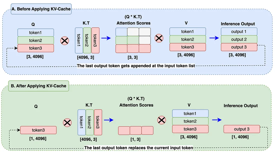Fig 1. KV-cache explanation. Image from internet

从新梳理一下，在计算第一个token的时候，cache下 \(K_{cache} =V_{cache}\)

然后当预测第二个token的时候，计算新predict的token的\(K\)和\(Q\), \(Q_{new} = [1.1,0.9,1.3,1.1]\)， \(K_{new} = V_{new} = [1.1,0.9,1.3,1.1]\)。这样就得到新的 \(K_{cache}\),

同样，因为我们的\(W\)设置，\(V_{cache}\) 也是这个矩阵。这样就可以算出新的attention weight为 \(Q_{new} \cdot K_{cache}^T / \sqrt{4} = [0.74, 1.66, 2.34]\)

import torch

# Setup
W_Q = W_K = W_V = torch.eye(4)
embeddings = {0: torch.tensor([0.1, 0.3, 0.3, 0.5]),  # "it"
              1: torch.tensor([0.6, 0.6, 0.8, 0.8]),  # "is"
              2: torch.tensor([1.1, 0.9, 1.3, 1.1])}  # "sunny"

# Initialize cache
K_cache = torch.empty(0, 4)
V_cache = torch.empty(0, 4)

def self_attention_with_cache(X_new, K_cache, V_cache):
    Q = X_new @ W_Q
    K_new = X_new @ W_K
    V_new = X_new @ W_V
    K_cache = torch.cat([K_cache, K_new], dim=0)
    V_cache = torch.cat([V_cache, V_new], dim=0)
    scores = Q @ K_cache.T / (4 ** 0.5)
    weights = torch.softmax(scores, dim=-1)
    output = weights @ V_cache
    return output, K_cache, V_cache

# Process prompt
prompt = torch.stack([embeddings[0], embeddings[1]])
for i in range(prompt.size(0)):
    output, K_cache, V_cache = self_attention_with_cache(prompt[i:i+1], K_cache, V_cache)
print("Prompt output:", output)

# Predict next token
new_token = embeddings[2].unsqueeze(0)
output, K_cache, V_cache = self_attention_with_cache(new_token, K_cache, V_cache)
print("Next token output:", output)